8. Response of linear systems to random excitation

Let us return to the linear single-degree-of-freedom system (see the chapter Properties of a linear time-invariant system):

\[ \underbrace{f(t)}_{\textrm{Excitation}}\to {\fbox{System}}\to \underbrace{x(t)}_{\textrm{Response}}. \]

We compute the response to deterministic excitation with the help of convolution:

\[ x(t) = \int_{-\infty}^{t}\,f(\tau)\,h(t-\tau)\,\textrm{d} \tau = \int_{0}^{+\infty}\,h(\tau)\,f(t-\tau)\,\textrm{d} \tau, \]

where \(h(t)\) is the impulse response function that defines the linear system.

Mean value of the response

In what follows, we will assume that the excitation \(f(t)\) is random. Let us first compute the expected mean value of the response. We must use the expectation operator \(E[]\):

\[ \mu_x = E[x(t)] = E\Big[ \int_{0}^{+\infty}\,h(\tau)\,f(t-\tau)\,\textrm{d} \tau \Big], \]

since the random value is only in the excitation \(f(t)\), it follows:

\[ \mu_x = \int_{0}^{+\infty}\,h(\tau)\,E\big[f(t-\tau)\big]\,\textrm{d} \tau = \int_{0}^{+\infty}\,h(\tau)\,\mu_f\,\textrm{d} \tau , = \mu_f\,\int_{0}^{+\infty}\,h(\tau)\,\textrm{d} \tau . \]

We can conclude:

Note

if we observe a process that has a mean value equal to zero at the input/excitation, then the mean value of the response will also be equal to zero (regardless of the impulse response function):

\[ \mu_x = \mu_f\,\int_{0}^{+\infty}\,h(\tau)\,\textrm{d} \tau . \]

Autocorrelation function

Here we want to answer the question of how the autocorrelation function of the excitation \(R_{ff}(\tau)\) is related to the autocorrelation function of the response \(R_{xx}(\tau)\); let us look at the details:

\[\begin{split} \begin{split} R_{xx}(\tau)&=E\big[x(t)\,x(t+\tau)\big]\\ &=E\Big[\int_{0}^{+\infty}\int_{0}^{+\infty}\,h(\tau_1)\,f(t-\tau_1)\,\,h(\tau_2)\,f(t+\tau-\tau_2)\,\textrm{d} \tau_1\,\textrm{d} \tau_2\Big]. \end{split} \end{split}\]

We continue with the derivation: since \(h(t)\) is uniquely determined, \(h(t)=E[h(t)]\):

\[ R_{xx}(\tau) =\int_{0}^{+\infty}\int_{0}^{+\infty}\,h(\tau_1)\,h(\tau_2)\,E\Big[f(t-\tau_1)\,f(t+\tau-\tau_2)\Big]\,\textrm{d} \tau_1\,\textrm{d} \tau_2. \]

We use the substitution \(t_1=t-\tau_1\), from which it follows that \(E\Big[f(t-\tau_1)\,f(t+\tau-\tau_2)\Big]=E\Big[f(t_1)\,f(t_1+\tau_1+\tau-\tau_2)\Big]=R_{ff}(\tau+\tau_1-\tau_2)\) and then:

\[ R_{xx}(\tau) =\int_{0}^{+\infty}\int_{0}^{+\infty}\,h(\tau_1)\,h(\tau_2)\,R_{ff}(\tau+\tau_1-\tau_2)\,\textrm{d} \tau_1\,\textrm{d} \tau_2. \]

Let us now make the transition into the frequency domain:

\[\begin{split} \begin{split} S_{xx}(f) &= \int_{-\infty}^{+\infty}R_{xx}(\tau)\,\mathrm{e}^{-\textrm{i}\,2\pi\,f\,\tau}\,\textrm{d}\tau\\ &= \underbrace{\int_{0}^{+\infty}\,h(\tau_1)\,\mathrm{e}^{+\textrm{i}\,2\pi\,f\,\tau_1}\,\textrm{d} \tau_1}_{H^*(f)}\, \underbrace{\int_{0}^{+\infty}\,h(\tau_2)\,\mathrm{e}^{-\textrm{i}\,2\pi\,f\,\tau_2}\,\textrm{d} \tau_2}_{H(f)}\, \underbrace{\int_{-\infty}^{+\infty}R_{ff}(u)\,\mathrm{e}^{-\textrm{i}\,2\pi\,f\,u}\,\textrm{d} u}_{S_{ff}(f)}. \end{split} \end{split}\]

Note: in the above expression we used the substitution: \(u=\tau+\tau_1-\tau_2\) and consequently \(\mathrm{e}^{-\textrm{i}\,2\pi\,f\,\tau}=\mathrm{e}^{-\textrm{i}\,2\pi\,f\,(u-\tau_1+\tau_2)}\) and then separated the integration variables.

The final result is:

Note

the auto power spectral density on the response side is defined as:

\[ S_{xx}(f) = H^*(f)\,H(f)\,S_{ff}(f), \]

where \({}^*\) denotes the complex conjugate value.

Cross-correlation function

Let us now look at the cross-correlation function \(R_{fx}(\tau)\) of the excitation \(f(t)\) and the response \(x(t)\):

\[\begin{split} \begin{split} R_{fx}(\tau)&=E\big[f(t)\,x(t+\tau)\big]\\ &=E\Big[\int_{0}^{+\infty}f(t)\,h(\tau_1)\,f(t+\tau-\tau_1)\,\textrm{d} \tau_1\Big]\\ &=\int_{0}^{+\infty}h(\tau_1)\,E\big[f(t)\,f(t+\tau-\tau_1)\big]\,\textrm{d} \tau_1\\ &=\int_{0}^{+\infty}h(\tau_1)\,R_{ff}(\tau-\tau_1)\,\textrm{d} \tau_1. \end{split} \end{split}\]

Let us now make the transition into the frequency domain:

\[\begin{split} \begin{split} S_{fx}(f) &= \int_{-\infty}^{+\infty}R_{fx}(\tau)\,\mathrm{e}^{-\textrm{i}\,2\pi\,f\,\tau}\,\textrm{d}\tau\\ &= \underbrace{\int_{0}^{+\infty}\,h(\tau_1)\,\mathrm{e}^{-\textrm{i}\,2\pi\,f\,\tau_1}\,\textrm{d} \tau_1}_{H(f)}\, \underbrace{\int_{-\infty}^{+\infty}R_{ff}(u)\,\mathrm{e}^{-\textrm{i}\,2\pi\,f\,u}\,\textrm{d} u}_{S_{ff}(f)}. \end{split} \end{split}\]

Note: in the above expression we used the substitution: \(u=\tau-\tau_1\) and consequently \(\mathrm{e}^{-\textrm{i}\,2\pi\,f\,\tau}=\mathrm{e}^{-\textrm{i}\,2\pi\,f\,(u+\tau_1)}\) and then separated the integration variables. The final result is:

Note

the cross power spectral density is defined as:

\[ S_{fx}(f) = H(f)\,S_{ff}(f). \]

Unlike the auto-spectral density, the cross-spectral density preserves the phase information!

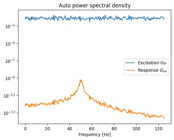
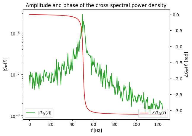
Example 1

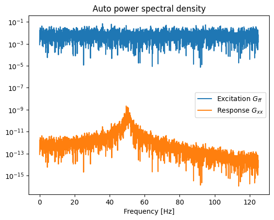
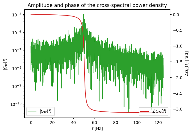
With the help of the example below, we will look at the auto- and cross-spectral density on randomly generated, normally distributed data.

Show code cell source

Hide code cell source

import numpy as np
import matplotlib.pyplot as plt

rng = np.random.default_rng(0)
N = 5000
fs = 250
dt = 1./fs
f = rng.normal(size=N)
time = np.arange(N)*dt

F = np.fft.rfft(f)
scale = 1.0 / (fs*N)
freq = np.fft.rfftfreq(N, d=dt)
G_ff = 2*scale*np.abs(F.conj()*F)

def alpha(freq, m, k, c):
    """
    Frequency response function of a linear oscillator.
    """
    omega = 2*np.pi*freq
    return 1 / (-omega**2*m + 1j*omega*c + k)

H = alpha(freq, m=1,k=1e5,c=10)
G_xx = np.abs(H.conj()*H*G_ff)
G_fx = H*G_ff

plt.title('Auto power spectral density')
plt.semilogy(freq, G_ff, label='Excitation $G_{ff}$')
plt.semilogy(freq, G_xx, label='Response $G_{xx}$')
plt.xlabel('Frequency [Hz]')
plt.legend()
plt.show()


fig, ax = plt.subplots()
ax.set_title('Amplitude and phase of the cross-spectral power density')
ax.semilogy(freq, np.abs(G_fx), color='C2', label='$|G_{fx}(f)|$')
ax.legend(loc=3)
ax.set_xlabel('$f$ [Hz]')
ax.set_ylabel('$|G_{fx}(f)|$')
ax2 = ax.twinx() 
ax2.plot(freq, np.angle(G_fx), color='C3', label='$\\angle G_{fx}(f)$')
ax2.set_xlabel('$f$ [Hz]')
ax2.set_ylabel('$\\angle G_{fx}(f)$ [rad]')
ax2.legend(loc=4)
plt.show()

Example 2

Let us also look at how we average the spectral density and thereby reduce the frequency resolution and the amplitude scatter.

Show code cell source

Hide code cell source

from scipy import signal

segments = 10
N_ = N//segments
win = signal.windows.boxcar(N_)              # window
scale = 1.0 / (fs*(win*win).sum())

G_ff = np.zeros(N_//2+1, dtype=complex)

for i in range(segments):
    f_ = f[i*N_:(i+1)*N_]
    f_w = win*f_          # window
    F = np.fft.rfft(f_w)  # fft
    G_ff += scale*2*np.conj(F) * F / segments

G_ff = np.abs(G_ff)
freq = np.fft.rfftfreq(N_, d=dt)
H = alpha(freq, m=1, k=1e5, c=10)
G_xx = np.abs(H.conj()*H*G_ff)
G_fx = H*G_ff

plt.title('Auto power spectral density')
plt.semilogy(freq, G_ff, label='Excitation $G_{ff}$')
plt.semilogy(freq, G_xx, label='Response $G_{xx}$')
plt.xlabel('Frequency [Hz]')
plt.legend()
plt.show()


fig, ax = plt.subplots()
ax.set_title('Amplitude and phase of the cross-spectral power density')
ax.semilogy(freq, np.abs(G_fx), color='C2', label='$|G_{fx}(f)|$')
ax.legend(loc=3)
ax.set_xlabel('$f$ [Hz]')
ax.set_ylabel('$|G_{fx}(f)|$')
ax2 = ax.twinx() 
ax2.plot(freq, np.angle(G_fx), color='C3', label='$\\angle G_{fx}(f)$')
ax2.set_xlabel('$f$ [Hz]')
ax2.set_ylabel('$\\angle G_{fx}(f)$ [rad]')
ax2.legend(loc=4)
plt.show()

Coherence

Note

Coherence is defined as:

\[ \gamma_{fx}^2(f)=\frac{|G_{fx}(f)|^2}{G_{ff}(f)\,G_{xx}(f)} =\frac{|S_{fx}(f)|^2}{S_{ff}(f)\,S_{xx}(f)} \]

and represents a measure of the linear relationship between the input (the excitation \(f\)) and the output (the response \(x\)) of the system.

Since:

\[ |\underbrace{S_{fx}(f)}_{\frac{1}{T}\, F^*(f) \, X(f)}|^2\le \underbrace{S_{ff}(f)}_{\frac{1}{T}\, F^*(f) \, F(f)}\,\overbrace{S_{xx}(f)}^{\frac{1}{T}\, X^*(f) \, X(f)}, \]

the coherence \(\gamma_{fx}^2(f)\) lies in the range from 0 to 1:

\[ 0\le\gamma_{fx}^2(f)\le 1. \]

If the coherence is 0, this means that the excitation and the response are not related; if the coherence is 1, then the excitation and the response are linearly dependent. A deviation from 1 is also measured when we have noise in the measurement, consider a nonlinear system, or the response is (also) a consequence of other excitations and not only \(f(t)\).

Estimators of the frequency response function

The frequency response function (FRF) characterizes a dynamic system; we already got to know the different forms of the frequency response function theoretically in the chapter Frequency response function. Here we will look at how the FRF is estimated on the basis of measured data, and in doing so we will limit ourselves to systems with one (simultaneous) excitation and one (simultaneous) response (these are the so-called SISO systems: single input, single output).

A linear time-invariant SISO system can be represented by a block diagram, as we have done in the figure below, where \(f(t)\) is the excitation force, \(h(t)\) the impulse response function and \(x(t)\) the response; \(F(\omega)\), \(\alpha(\omega)\) and \(X(\omega)\) are their counterparts in the frequency domain.

For a random process, the FRF is defined by \(\alpha(\omega)=S_{fx}(\omega)/S_{ff}(\omega)\), where \(S_{ff}(\omega)\) and \(S_{fx}(\omega)\) are the auto- and cross power spectral densities.

The figure below shows a SISO system, where \(u(t)\) and \(v(t)\) are the true input (excitation) and the true output (response) of the system. \(m(t)\) represents the measured noise at the input \(f(t)\) and \(n(t)\) the measured noise at the output \(x(t)\). The capital letters are the corresponding frequency-domain quantities.

Measurement noise is always present and prevents us from measuring the actual values that enter or leave the system. The figure shows that, in reality, it is not possible to measure the actual input to the system \(u(t)\), nor is it possible to measure the actual output from the system \(v(t)\). Instead, we measure the input with noise:

\[ f(t)=u(t)+m(t) \]

and the output with noise:

\[ x(t)=v(t)+n(t). \]

For arbitrary correlations between the signals \(u(t)\) and \(v(t)\) and the noise \(m(t)\) and \(n(t)\), we can define the auto- and cross power spectral densities:

\[\begin{split} \begin{split} S_{ff}(\omega) &= S_{uu}(\omega) + S_{mm}(\omega) + S_{mu}(\omega) + S_{um}(\omega),\\ S_{xx}(\omega) &= S_{vv}(\omega) + S_{nn}(\omega) + S_{nv}(\omega) + S_{vn}(\omega),\\ S_{fx}(\omega) &= S_{uv}(\omega) + S_{un}(\omega) + S_{mv}(\omega) + S_{mn}(\omega). \end{split} \end{split}\]

The input \(u(t)\) and the output \(v(t)\) of the system are related by means of the FRF:

\[\begin{split} \begin{split} S_{vv}(\omega)&=|\alpha(\omega)|^2\,S_{uu}(\omega),\\ S_{uv}(\omega)&=\alpha(\omega)\,S_{uu}(\omega). \end{split} \end{split}\]

In what follows, we will try to estimate the actual frequency response function from the noisy measurements (\(f(t)=u(t)+m(t)\) and \(x(t)=v(t)+n(t)\)).

Estimator \(\hat{H}_1\)

When measuring the excitation \(f(t)\) and the response \(x(t)\), the latter usually covers a larger dynamic range (in the measurement we have relatively large values and also relatively small ones) and is therefore more sensitive to measurement noise. Because of this, we assume that there is no input noise (\(m(t)=0\)); consequently:

\[ S_{mm}(\omega)=0,\quad S_{mn}(\omega)=0,\quad S_{mu=0}(\omega)=0,\quad S_{mv}(\omega)=0 \]

and that the output noise \(n(t)\) is not correlated with the system, so:

\[ S_{un}(\omega)=0. \]

Consequently, the auto- and cross-spectral densities simplify:

\[\begin{split} \begin{split} S_{ff}(\omega) &= S_{uu}(\omega),\\ S_{xx}(\omega) &= S_{vv}(\omega) + S_{nn}(\omega),\\ S_{fx}(\omega) &= S_{uv}(\omega). \end{split} \end{split}\]

From the last equation, we can estimate the actual FRF on the basis of the measured data (\(x(t)\) and \(f(t)\)): \(S_{fx}(\omega)= S_{uv}(\omega)\). With the help of the relation \(S_{uv}(\omega)=\alpha(\omega)\,S_{uu}(\omega)\), we can estimate the FRF as:

Note

estimator \(\hat{H}_1(\omega)\):

\[ \begin{split} \hat{H}_1(\omega)&=\hat{\alpha}_1(\omega)=\frac{\hat{S}_{fx}(\omega)}{\hat{S}_{ff }(\omega)}, \end{split} \]

where we used the symbol \(\hat{~}\) to denote an estimate from a measurement. Here it is important that we obtain the auto- \(\hat{S}_{ff}(\omega)\) and cross-spectral \(\hat{S}_{fx} (\omega)\) power densities by averaging the random process (see the example below).

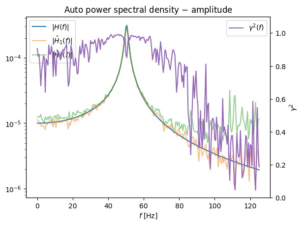
To estimate the quality and linearity of the measurement, we also need the coherence:

\[ \begin{split} \hat{\gamma}_{fx}^2(\omega)&=\frac{|\hat{S}_{fx}(\omega)|^2}{\hat{S}_{ff}(\omega)\,\big(\underbrace{{S}_{vv}(\omega)+S_{nn}(\omega)}_{\hat{S}_{xx}(\omega)}\big)}, \end{split} \]

which shows that the output noise \(S_{nn}(\omega)\) reduces the coherence and thereby the quality of the estimated FRF.

If the excitation noise \(m(t)\) cannot be neglected, then \(S_{ff}(\omega)=S_{uu}(\omega)+S_{mm}(\omega)\) and:

\[ \begin{split} \hat{H}_1(\omega)&=\frac{\hat{S}_{fx}(\omega)}{\hat{S}_{uu}(\omega)+\hat{S}_{mm}(\omega)}. \end{split} \]

It follows that the estimator \(\hat{H}_1\), because of the input noise, underestimates the true FRF \(\alpha(\omega)=S_{uv}(\omega)/S_{uu}(\omega)\).

Estimator \(\hat{H}_2\)

Here we investigate the estimation of the FRF when the measurement noise on the excitation side cannot be neglected, but is not correlated with the system. Furthermore, we assume that the noise on the response side can be neglected (\(n(t)=0\)); consequently:

\[\begin{split} \begin{split} S_{ff}(\omega) &= S_{uu}(\omega) + S_{mm}(\omega),\\ S_{xx}(\omega) &= S_{vv}(\omega),\\ S_{fx}(\omega) &= S_{uv}(\omega). \end{split} \end{split}\]

We use:

\[\begin{split} \begin{split} S_{xx}(\omega)&=S_{vv}(\omega)\\ &=|\alpha(\omega)|^2\,S_{uu}(\omega)\\ &=\alpha(\omega)\,\alpha(\omega)^*\,S_{uu}(\omega)\\ &=\alpha(\omega)\,S_{xf}(\omega), \end{split} \end{split}\]

where in the last line we used \(S_{xf}(\omega)=S_{vu}(\omega)=\alpha(\omega)^*\,S_{uu}(\omega)\).

Consequently, we derived an estimator for estimating the FRF:

Note

estimator \(\hat{H}_2(\omega)\):

\[ \begin{split} \hat{H}_2(\omega)&=\hat{\alpha}_2(\omega)=\frac{\hat{S}_{xx}(\omega)}{\hat{S}_{xf}(\omega)}. \end{split} \]

The coherence function becomes:

\[ \begin{split} \hat{\gamma}_{fx}^2(\omega)&=\frac{|\hat{S}_{fx}(\omega)|^2}{\big(\underbrace{{S}_{uu}(\omega)+{S}_{mm}(\omega)}_{\hat{S}_{ff}(\omega)}\big)\,\hat{S}_{xx}(\omega)}, \end{split} \]

which shows that noise on the excitation side also reduces the coherence and thereby the quality of the estimated FRF.

We can observe that if we divide the estimator \(\hat{H}_1\) by the estimator \(\hat{H}_2\), we obtain the coherence estimator:

\[ \begin{split} \hat{\gamma}_{fx}^2(\omega)&=\frac{\hat{H}_1(\omega)}{\hat{H}_2(\omega)}. \end{split} \]

If the noise on the response side \(n(t)\) cannot be neglected, then \(S_{xx}(\omega)=S_{vv}(\omega)+S_{nn}(\omega)\) and:

\[ \begin{split} \hat{H}_2(\omega)&=\frac{\hat{S}_{vv}(\omega)+\hat{S}_{nn}(\omega)}{\hat{S}_{xf}(\omega)}. \end{split} \]

In the case of noise on the response, the estimator \(\hat{H}_2(\omega)\) therefore overestimates the true FRF \(\alpha(\omega)\).

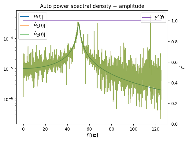
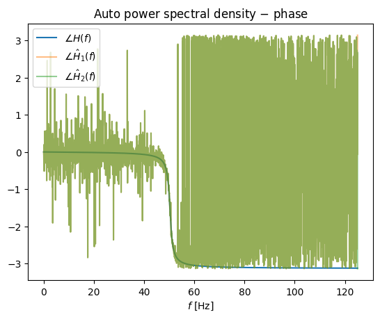
Example 1

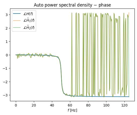
In the example below we can look at the use of the estimators \(H_1\) and \(H_2\) for estimating the frequency response function.

Show code cell source

Hide code cell source

import numpy as np
import matplotlib.pyplot as plt

rng = np.random.default_rng(0)
fs = 250
N = 5000
dt = 1./fs
time = np.arange(N)*dt

SNR_f = 20 # 20 dB means the ratio between the variance of the signal and the noise is 10
SNR_x = 20

σ_u = 1
σ_m = σ_u/10**(SNR_f/20) # based on the definition 20*np.log10(σ_u/σ_m)

u = rng.normal(size=N, scale=σ_u)
m = rng.normal(size=N, scale=σ_m)

f = u + m # measured excitation in time

scale = 1.0 / (fs*N)
U = np.fft.rfft(u) # actual excitation of the system
F = np.fft.rfft(f) # measured excitation of the system
freq = np.fft.rfftfreq(N, d=dt)

G_uu = 2*scale*np.abs(U.conj()*U)
G_ff = 2*scale*np.abs(F.conj()*F)

def alpha(freq, m, k, c):
    """
    Frequency response function of a linear oscillator.
    """
    omega = 2*np.pi*freq
    return 1 / (-omega**2*m + 1j*omega*c + k)

H = alpha(freq, m=1,k=1e5,c=10)
V = H*U                      # response without noise
v = np.fft.irfft(V)        # actual response in time
σ_n = np.std(v)/10**(SNR_x/20) # based on the definition 20*np.log10(σ_v/σ_n)
n = rng.normal(size=N, scale=σ_n)

x = v + n            # measured response of the system
X = np.fft.rfft(x) # measured excitation of the system

G_fx = 2*scale*F.conj()*X
G_xx = 2*scale*np.abs(X.conj()*X)
G_xf = G_fx.conj()

H1 = G_fx/G_ff
H2 = G_xx/G_xf
γ2 = np.abs(H1/H2)

fig, ax = plt.subplots()
ax.set_title('Auto power spectral density $-$ amplitude')
ax.semilogy(freq, np.abs(H), label='$|H(f)|$')
ax.semilogy(freq, np.abs(H1), label='$|\\hat H_1(f)|$', alpha=0.5)
ax.semilogy(freq, np.abs(H2), label='$|\\hat H_2(f)|$', alpha=0.5)
ax.set_xlabel('$f$ [Hz]')
ax.legend(loc=2)
ax2 = ax.twinx() 
ax2.plot(freq, γ2, 'C4', label='$\\gamma^2(f)$')
ax2.set_xlabel('$f$ [Hz]')
ax2.set_ylabel('$\\gamma^2$')
ax2.set_ylim(0,1.1)
ax2.legend(loc=1)
plt.show()

fig, ax = plt.subplots()
ax.set_title('Auto power spectral density $-$ phase')
ax.plot(freq, np.angle(H), label='$\\angle H(f)$')
ax.plot(freq, np.angle(H1), label='$\\angle\\hat H_1(f)$', alpha=0.5)
ax.plot(freq, np.angle(H2), label='$\\angle\\hat H_2(f)$', alpha=0.5)
ax.set_xlabel('$f$ [Hz]')
ax.legend()
plt.show()

Example 2

We continue with the example and add segment averaging; with this we reduce the frequency resolution and also the scatter of the frequency response function estimator.

Show code cell source

Hide code cell source

from scipy import signal

segments = 10
N_ = N//segments
win = signal.windows.hann(N_)              # window
scale = 1.0 / (fs*(win*win).sum())

G_fx = np.zeros(N_//2+1, dtype=complex) # clearing
G_ff = np.zeros(N_//2+1, dtype=complex)
G_xf = np.zeros(N_//2+1, dtype=complex)
G_xx = np.zeros(N_//2+1, dtype=complex)


for i in range(segments):
    f_ = f[i*N_:(i+1)*N_]
    x_ = x[i*N_:(i+1)*N_]
    f_w = win*f_          # window
    x_w = win*x_
    F = np.fft.rfft(f_w)  # fft
    X = np.fft.rfft(x_w)
    G_fx += scale*2*np.conj(F) * X / segments # the estimators of the auto- and cross-spectrum must be averaged
    G_ff += scale*2*np.conj(F) * F / segments 
    G_xf += scale*2*np.conj(X) * F / segments 
    G_xx += scale*2*np.conj(X) * X / segments

freq = np.fft.rfftfreq(N_, d=dt)
H = alpha(freq, m=1, k=1e5, c=10)

H1 = G_fx/G_ff
H2 = G_xx/G_xf
γ2 = np.abs(H1/H2)

sel = freq>=0
#sel = np.logical_and(freq>40, freq<60)    # to view what happens at the natural frequency
fig, ax = plt.subplots()
ax.set_title('Auto power spectral density $-$ amplitude')
ax.semilogy(freq[sel], np.abs(H[sel]), label='$|H(f)|$')
ax.semilogy(freq[sel], np.abs(H1[sel]), label='$|\\hat H_1(f)|$', alpha=0.5)
ax.semilogy(freq[sel], np.abs(H2[sel]), label='$|\\hat H_2(f)|$', alpha=0.5)
ax.set_xlabel('$f$ [Hz]')
ax.legend(loc=2)
ax2 = ax.twinx() 
ax2.plot(freq[sel], γ2[sel], 'C4', label='$\\gamma^2(f)$')
ax2.set_xlabel('f [Hz]')
ax2.set_ylabel('$\\gamma^2$')
ax2.set_ylim(0,1.1)
ax2.legend(loc=1)
plt.show()

fig, ax = plt.subplots()
ax.set_title('Auto power spectral density $-$ phase')
ax.plot(freq[sel], np.angle(H[sel]), label='$\\angle H(f)$')
ax.plot(freq[sel], np.angle(H1[sel]), label='$\\angle\\hat H_1(f)$', alpha=0.5)
ax.plot(freq[sel], np.angle(H2[sel]), label='$\\angle\\hat H_2(f)$', alpha=0.5)
ax.set_xlabel('$f$ [Hz]')
ax.legend()
plt.show()