6. The discrete Fourier transform

Earlier we got to know the Fourier transform for sampled data (see the chapter Uniform time sampling), where we sample with step \(\Delta t\,n\) and \(n\in\mathbb{Z}\) goes from \(-\infty\) to \(+\infty\). When we have a finite number of sampled data (\(N\)) and \(n=[0,1,\dots,N-1]\), we use the discrete Fourier transform (DFT).

Note

Discrete Fourier transform:

\[ X_k = \sum_{n=0}^{N-1} x_n\,\mathrm{e}^{-\mathrm{i}\,2\pi\,k\,n/N}, \]

where \(x_n = x(n\,\Delta t)\) and \(X_k=X(k/(N\,\Delta t))\). Since the DFT is periodic with \(1/\Delta t\) (\(X_k=X_{k+N}\)), only \(N\) terms need to be computed, i.e. \(k=[0,1,\dots\,N-1]\).

That \(X_k=X_{k+N}\) holds, we prove with:

\[ \mathrm{e}^{-\mathrm{i}\,2\pi\,k\,n/N}=\mathrm{e}^{-\mathrm{i}\,2\pi\,n\,(k+N)/N}=\mathrm{e}^{-\mathrm{i}\,2\pi\,n\,k/N}\,\underbrace{\mathrm{e}^{-\mathrm{i}\,2\pi\,n\,N/N}}_{=\cos(-2\pi\,n)=1}. \]

We derive the inverse DFT by multiplying the above equation by \(\mathrm{e}^{\mathrm{i}\,2\pi\,k\,r/N}\) and then summing over \(k\):

\[ \sum_{k=0}^{N-1}X_k\,\mathrm{e}^{\mathrm{i}\,2\pi\,k\,r/N} = \sum_{k=0}^{N-1}\sum_{n=0}^{N-1} x_n\,\mathrm{e}^{-\mathrm{i}\,2\pi\,k\,n/N}\,\mathrm{e}^{\mathrm{i}\,2\pi\,k\,r/N}, \]

then on the right-hand side we swap the order of the sum and find:

\[\begin{split} \sum_{k=0}^{N-1} \mathrm{e}^{-\mathrm{i}\,2\pi\,k\,(n-r)/N}= \begin{cases} 1; &\quad n=r,\\ 0 &\quad\textrm{otherwise.} \end{cases} \end{split}\]

It follows:

\[ \sum_{n=0}^{N-1}x_r\,1=x_r\,N \]

and then we derive:

\[ \sum_{k=0}^{N-1}X_k\,\mathrm{e}^{\mathrm{i}\,2\pi\,k\,r/N} = x_r\,N. \]

Note

Inverse discrete Fourier transform:

\[ x_n = \frac{1}{N} \sum_{k=0}^{N-1} X_k\,\mathrm{e}^{\mathrm{i}\,2\pi\,k\,n/N}, \]

since:

\[ \mathrm{e}^{\mathrm{i}\,2\pi\,k\,n/N}=\mathrm{e}^{\mathrm{i}\,2\pi\,k\,(n+N)/N}=\mathrm{e}^{\mathrm{i}\,2\pi\,k\,n/N}\,\underbrace{\mathrm{e}^{\mathrm{i}\,2\pi\,k\,N/N}}_{=\cos(2\pi\,k)=1}. \]

Note

We find that \(x_n\) is a periodic series \(x_n=x_{n+N}\). We indeed started with time-sampled data \(x_n\), which are not periodic; but the result obtained with the inverse DFT is periodic.

Fast Fourier transform

The fast Fourier transform (FFT) is the name of a numerical algorithm for the discrete Fourier transform. The DFT has a numerical complexity proportional to \(N^2\), which we write as \(\mathcal{O}(N^2)\). James Cooley and John Tukey are considered the authors of the fast Fourier transform; they published the algorithm in 1965 (see source), and it later turned out that a similar algorithm had already been discovered, significantly earlier, in unpublished work from 1805, by Carl Friedrich Gauss. Compared to the DFT, the algorithm is numerically significantly faster: \(\mathcal{O}(N\log(N))\); since the numerical complexity does not grow quadratically with the number of elements \(N\), this significantly increased the usefulness of the DFT. Some consider the FFT algorithm to be one of the most important algorithms, since it had (and still has) a very important socio-economic impact. As an interesting fact, we can mention here that the algorithm was not patented (see source). Because of the symmetry in the data, the computation speed is highest when the number of samples is equal to \(2^n\), where \(n\in\mathbb{Z}\).

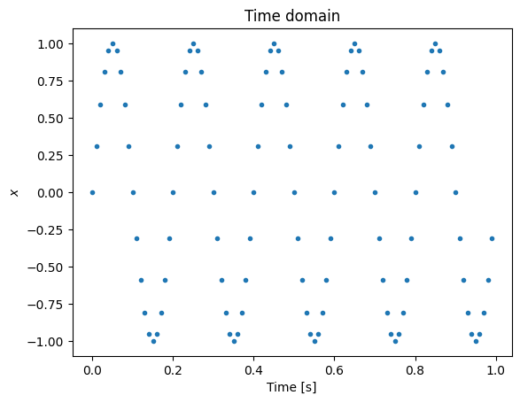
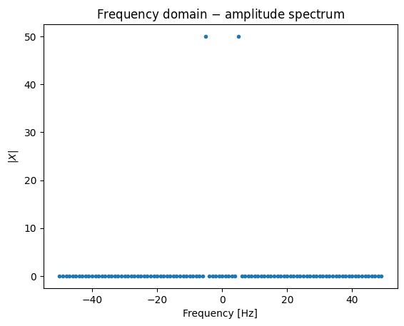
The discrete Fourier transform is documented in the numpy package here, and we will first look at it on the example below of a sinusoid with amplitude A, frequency fr, sampling frequency fs and sampling length N, which will be equal to the sampling frequency (we will therefore sample 1 second). We will perform the DFT with the method numpy.fft.fft() (documentation).

import numpy as np

A = 1
fr = 5
fs = 100 
N = 100
dt = 1/fs
t = np.arange(N)*dt
x = A*np.sin(2*np.pi*fr*t)

X = np.fft.fft(x)
freq = np.fft.fftfreq(len(x), d=dt)

The sinusoid has only one non-zero frequency component:

(X[freq==fr], np.abs(X[freq==fr]))

(array([-1.61933301e-14-50.j]), array([50.]))

Show code cell source

Hide code cell source

import matplotlib.pyplot as plt

plt.title('Time domain')
plt.plot(t, x, '.')
plt.xlabel('Time [s]')
plt.ylabel('$x$')
plt.show()

plt.title('Frequency domain $-$ amplitude spectrum')
plt.plot(freq, np.abs(X), '.')
plt.xlabel('Frequency [Hz]')
plt.ylabel('$|X|$')
plt.show()

Fourier series and the discrete Fourier transform

The discrete Fourier transform is very closely related to Fourier series. The connection can be quickly revealed if we assume a discrete time series \(x_i=x(\Delta t\,i)\), where \(\Delta t\) is a constant time step, \(i=0,1,\dots,N-1\) and \(T_p=N\,\Delta t\); it follows:

\[\begin{split} \begin{split} c_k &= \frac{1}{T_p}\,\int_0^{T_p} x(t)\,\mathrm{e}^{-\mathrm{i}\,2\pi\,k\,t/T_p}\,\mathrm{d}t\\ &= \frac{1}{N\,\Delta t}\,\sum_{n=0}^{N-1} x(n\,\Delta t)\,\mathrm{e}^{-\mathrm{i}\,2\pi\,k\,\Delta t\,n/(N\,\Delta t)}\,\Delta t\\ &= \frac{1}{N}\,\underbrace{\sum_{n=0}^{N-1} x(n\,\Delta t)\,\mathrm{e}^{-\mathrm{i}\,2\pi\,k\,n/N}}_{X_k}\\ &= \frac{X_k}{N}.\\ \end{split} \end{split}\]

It must be emphasized that in general \(X_k/N\ne c_k\), since the DFT is based on a finite series and therefore \(X_k\) is a periodic series.

When comparing the DFT and Fourier series, an error in understanding the period (especially the last discrete point) often arises. In the example of the sinusoid above, the time point at t = 1 is explicitly not included; but it is implicitly included, since we learned above that the sampled data are periodic and \(x_n=x_{n+N}\). Let us look at this detail more closely; the terms of the Fourier series are defined as:

\[ c_n = \frac{1}{T_p}\,\int_0^{T_p} x(t)\,\mathrm{e}^{-\mathrm{i}\,2\pi\,n\,t/T_p}\,\mathrm{d}t. \]

We compute the Fourier coefficient for the frequency fr:

import sympy as sym

t, fr, Tp, A = sym.symbols('t, fr, Tp, A')
π = sym.pi
i = sym.I

data = {fr: 5, A:1, Tp:1}

x = sym.sin(2*π*fr*t)
c = 1/Tp*sym.integrate(x*sym.exp(-i*2*π*fr*t/Tp), (t,0,Tp))

c.subs(data)

\[\displaystyle - \frac{i}{2}\]

We arrive at the same result via the DFT, but the last time point is explicitly not included:

import numpy as np

A = 1
fr = 5
fs = 100 
N = 100
# The `fs` below results in the last point being included. The result will be wrong!
#fs = 100/1.01010101010101
dt = 1/fs
t = np.arange(100)*dt
x = A*np.sin(2*np.pi*fr*t)

X_r = np.fft.rfft(x)
freq_r = np.fft.rfftfreq(len(x), d=dt)

c = X_r[freq_r==fr] / len(x)
c

array([-1.84965704e-16-0.5j])

Let us convince ourselves that the last time point is explicitly not included:

t[-3:]

array([0.97, 0.98, 0.99])

If, in the code above, we change fs or the number of points so that the last point is explicitly included, the result will not be equal to the one from Fourier series!

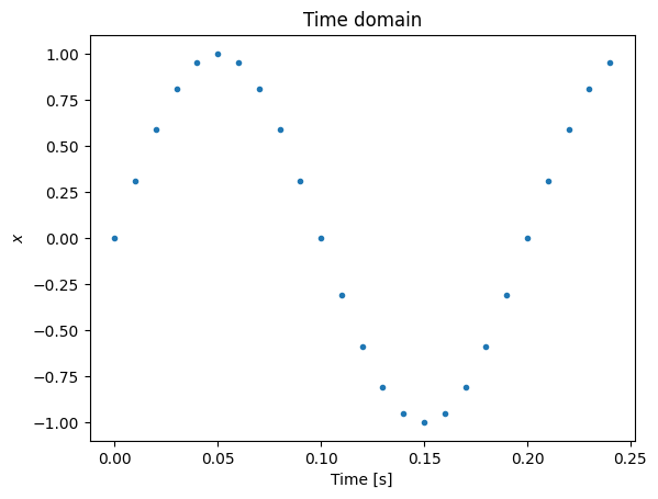
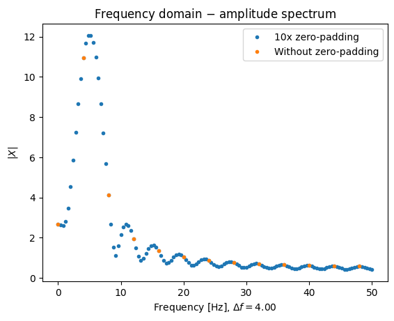
Frequency resolution and zero-padding

The frequency resolution of the DFT is defined by the length of the discrete time series \(x_i=x(\Delta t\,i)\), where \(\Delta t\) is a constant time step, \(i=0,1,\dots,N-1\); the length of such a series is therefore \(T_p=N\,\Delta t\), so it follows that the frequency resolution is:

\[ \Delta f= \frac{1}{N\,\Delta t}. \]

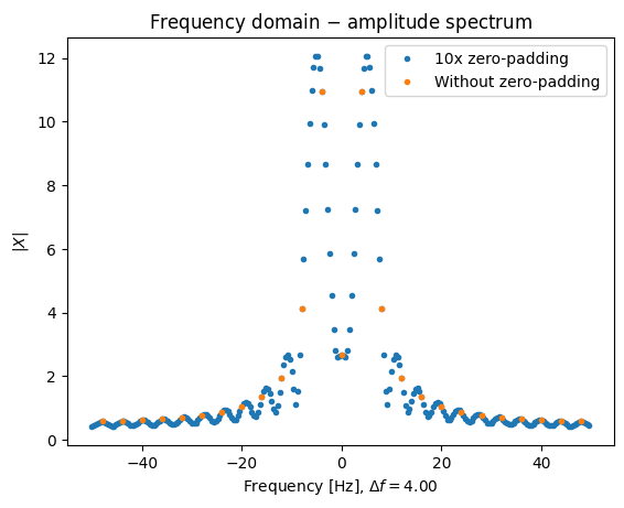
With a longer time series we could also have a better frequency resolution. When we cannot obtain additional points of the discrete series, we can increase the frequency resolution by zero-padding:

\[\begin{split} \tilde{x}_n= \begin{cases} x_n;\quad & 0\le n\le N-1,\\ 0;\quad & N\le n\le L-1. \end{cases} \end{split}\]

It follows:

Note

discrete Fourier transform with zero-padding:

\[ \tilde{X}_k = \sum_{n=0}^{L-1} \tilde{x}_n\,\mathrm{e}^{-\mathrm{i}\,2\pi\,k\,n/L} = \sum_{n=0}^{N-1} x_n\,\mathrm{e}^{-\mathrm{i}\,2\pi\,k\,n/L}. \]

In this way we obtain the frequency resolution:

\[ \Delta f = \frac{1}{L\,\Delta t}, \]

but here it must be emphasized that this is only a frequency interpolation, which allows us a more detailed insight; we do not add new information by zero-padding. Similarly to the DFT, we can add zeros in the frequency domain and then, with the inverse discrete Fourier transform, obtain denser (interpolated) time data.

When zero-padding, we must pay attention to the normalization of the data; namely, we do not take the added zeros into account in the normalization.

The example below shows the use of zero-padding; with the help of the comments in the code, explore how it works.

Show code cell source

Hide code cell source

import numpy as np
import matplotlib.pyplot as plt


A = 1
fr = 5
fs = 100 
N = 25 # try 20 here (the sinusoid completes; the result without zero-padding is exact!)
k = 10 # zero-padding
dt = 1/fs
t = np.arange(N)*dt
x = A*np.sin(2*np.pi*fr*t)

X = np.fft.fft(x)
freq = np.fft.fftfreq(len(x), d=dt)

X_kx = np.fft.fft(x, n=k*N)
freq_kx = np.fft.fftfreq(k*N, d=dt)


plt.title('Time domain')
plt.plot(t, x, '.')
plt.xlabel('Time [s]')
plt.ylabel('$x$')
plt.show()

plt.title('Frequency domain $-$ amplitude spectrum')
plt.plot(freq_kx, np.abs(X_kx), '.', label=f'{k}x zero-padding')
plt.plot(freq, np.abs(X), '.', label='Without zero-padding')
plt.xlabel(f'Frequency [Hz], $\\Delta f=${1/(N*dt):3.2f}')
plt.ylabel('$|X|$')
plt.legend()
plt.show()

Symmetry of the DFT for real data

Note

For real data, in the frequency domain:

\[\begin{split} \begin{split} \textrm{Re}\big(X(k)\big)&=\textrm{Re}\big(X(N-k)\big),\\ \textrm{Im}\big(X(k)\big)&=-\textrm{Im}\big(X(N-k)\big),\\ |X(k)|&=|X(N-k)|,\\ \angle X(k)&=\angle X(N-k). \end{split} \end{split}\]

Since most engineering data in the time domain are real, it makes sense to use an appropriately adapted fast Fourier transform method; in the numpy package this is available via the call numpy.fft.rfft(). The inverse DFT is accessible via the methods numpy.fft.ifft or numpy.fft.irfft in the case of real data in the time domain.

We verify the stated properties in code in the numpy package (note: we add noise to the time signals so that the phase is not very close to 0):

import numpy as np

A = 1
fr = 5
fs = 100 
N = 10
dt = 1/fs
t = np.arange(N)*dt
np.random.seed(0)
x = A*np.sin(2*np.pi*fr*t) + np.random.normal(scale=A/2, size=N)

X = np.fft.fft(x)
freq = np.fft.fftfreq(len(x), d=dt)

X_r = np.fft.rfft(x)
freq_r = np.fft.rfftfreq(len(x), d=dt)

np.testing.assert_allclose(freq[1:N//2], -freq[:N//2:-1])
np.testing.assert_allclose(np.real(X[1:N//2]), np.real(X[:N//2:-1]))
np.testing.assert_allclose(np.imag(X[1:N//2]), -np.imag(X[:N//2:-1]))

np.testing.assert_allclose(np.abs(freq[:N//2+1]), freq_r)
np.testing.assert_allclose(np.real(X[:N//2+1]), np.real(X_r))
np.testing.assert_allclose(np.imag(X[:N//2+1]), np.imag(X_r), atol=1e-15)

And the above example with numpy.fft.rfft():

Show code cell source

Hide code cell source

import numpy as np
import matplotlib.pyplot as plt


A = 1
fr = 5
fs = 100 
N = 25 # try 20 here (the sinusoid completes; the result without zero-padding is exact!)
k = 10 # zero-padding
dt = 1/fs
t = np.arange(N)*dt
x = A*np.sin(2*np.pi*fr*t)

X = np.fft.rfft(x)
freq = np.fft.rfftfreq(len(x), d=dt)

X_kx = np.fft.rfft(x, n=k*N)
freq_kx = np.fft.rfftfreq(k*N, d=dt)


plt.title('Time domain')
plt.plot(t, x, '.')
plt.xlabel('Time [s]')
plt.ylabel('$x$')
plt.show()

plt.title('Frequency domain $-$ amplitude spectrum')
plt.plot(freq_kx, np.abs(X_kx), '.', label=f'{k}x zero-padding')
plt.plot(freq, np.abs(X), '.', label='Without zero-padding')
plt.xlabel(f'Frequency [Hz], $\\Delta f=${1/(N*dt):3.2f}')
plt.ylabel('$|X|$')
plt.legend()
plt.show()

Convolution of periodic data

We dealt with the convolution of functions in the case of the Fourier integral transform in the chapter Convolution of functions; here we will look at the particularities in the treatment of two periodic series (see the chapter Identification of the harmonic signals that make up a periodic signal) of equal length: \(x_n\) and \(y_n\):

\[ X_k = \sum_{n=0}^{N-1} x_n\,\mathrm{e}^{-\mathrm{i}\,2\pi\,k\,n/N}, \]

\[ Y_k = \sum_{n=0}^{N-1} y_n\,\mathrm{e}^{-\mathrm{i}\,2\pi\,k\,n/N}. \]

Similarly to functions, it also holds for periodic time series that the DFT of a convolution in the time domain is the product of the frequency transforms.

Note

Convolution of periodic data (also circular convolution):

\[ \textrm{DFT}\big\{x_n*y_n\big\}=X_k\,Y_k. \]

To emphasize that it is a circular convolution, the symbol \(\circledast\) is sometimes also used: \(x_n\circledast y_n\).

Emphasizing the periodicity of \(x_n\) and \(y_n\) is necessary, otherwise (circular) convolution is not possible; this will be clear from the following derivation:

\[\begin{split} \begin{split} \textrm{DFT}\big\{x_n\circledast y_n\big\}&=\textrm{DFT}\big\{\sum_r^{N-1}x_r\,y_{n-r}\big\}\\ &=\sum_n^{N-1}\sum_r^{N-1}x_r\,y_{n-r}\,\mathrm{e}^{-\textrm{i}\,2\pi\,n\,k/N}\\ &=\underbrace{\sum_r^{N-1}x_r\,\,\mathrm{e}^{-\textrm{i}\,2\pi\,r\,k/N}}_{X_k}\,\underbrace{\sum_n^{N-1}y_{n-r}\,\mathrm{e}^{-\textrm{i}\,2\pi\,(n-r)\,k/N}}_{Y_k}\\ &=X_k\,Y_k. \end{split} \end{split}\]

In the above derivation, it must be emphasized that the sum over \(r\) in the second-to-last line also includes the sum over \(n\), but since the sum over \(n\) is, because of periodicity, independent of \(r\), the sums over \(r\) and \(n\) can be performed independently. Because of the periodicity of \(y_n\), for every \(r\) it therefore holds that:

\[ \sum_n^{N-1}y_{n-r}\,\mathrm{e}^{-\textrm{i}\,2\pi\,(n-r)\,k/N}=\sum_n^{N-1}y_{n}\,\mathrm{e}^{-\textrm{i}\,2\pi\,n\,k/N}=Y_k. \]

If the series \(x_n\) and \(y_n\) were not periodic, the convolution of finite series would not be so simple.