7. Fundamentals of random processes

Dynamic loads are often not deterministic, but can have fully or partially random properties. An example of random loads are loads due to sea waves or road roughness. Such loads must be treated as random processes. In this chapter we will look at how we treat random loads and then successfully apply them to dynamic systems.

Random data differ from deterministic data, since they cannot be predicted exactly. However, with the help of an analysis of segments of random data, we can discern certain characteristics. For example, if we measure the surface roughness of one segment, we can, on this basis, infer with a certain probability the roughness of other segments. In describing random processes, an assumption about the distribution of the process is often used, such as for example the normal distribution.

Although it is possible to analyze a random process in the time domain, there are certain shortcomings in using such an approach. To adequately estimate the process, a sufficiently large number of sample measurements (or observations) in the time domain must be collected, which we then analyze as a group (an ensemble). As we will see later, the analysis of structural dynamics and random processes in the frequency domain is significantly more elegant.

We recommend that you look at some reference texts that deal in depth with random processes:

• Bendat and Piersol [2011],

• Newland [2012] and

• Shin and Hammond [2008].

Some of the content in this text is summarized from the book Slavič et al. [2020].

What is a random process?

A random process is defined by a combination of a probability density function (PDF) and a power spectral density (PSD).

The figure below shows an ensemble \(\left\{x_k(t)\right\}\) of sample functions (observations) \(x_k(t)\), where each observation \(k\) is composed of a random variable at time \(t_i\): \(x_k(t_i)\). As will be discussed in more detail later, the assumptions of stationarity and ergodicity significantly simplify the analysis of random data.

Normal distribution (Gaussian process)

The Gaussian distribution is often observed in various physical phenomena, and its prevalence is explained by the central limit theorem (Central limit theorem).

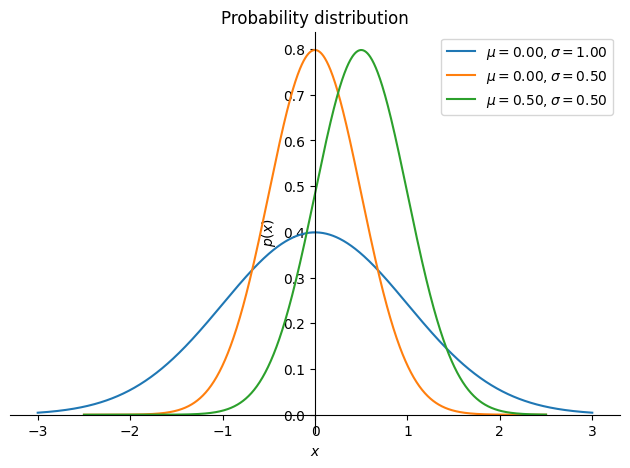
The probability density function (PDF) \(p(x)\) for a random process \(\left\{x(t_i)\right\}\) defines, at time \(t\), the probability of the amplitude \(x\); for a Gaussian process the PDF is defined as:

\[ p(x) = \frac{1}{\sigma \, \sqrt{2 \, \pi}} \, \mathrm{e}^{-\frac{(x-\mu)^2}{2 \,\sigma^2}}, \]

where \(\mu\) is the mean value, \(\sigma\) the standard deviation, and \(\sigma^2\) the variance. The mean value \(\mu\) and the variance \(\sigma^2\) determine the shape of the PDF and are often called the first moment and the second central moment; we compute them with the help of the probability density function:

\[ \mu = \int_{-\infty}^{+\infty} x \, p(x)\, \textrm{d} x, \]

\[ \sigma^2 = \int_{-\infty}^{+\infty} (x - \mu)^2 \, p(x)\, \textrm{d} x. \]

An example of different normal distributions is shown in the figure below.

Show code cell source

Hide code cell source

import sympy as sym
σ, μ, x, = sym.symbols('\\sigma, \\mu, x', real=True)
π = sym.pi

p = 1/(σ*sym.sqrt(2*π)) * sym.exp(-(x-μ)**2/(2*σ**2))

data = {σ: 1., μ: 0.}

p1 = sym.plot(p.subs(data), (x, -3*σ.subs(data), +3*σ.subs(data)), line_color='C0', 
              label=f'$\\mu={μ.subs(data):3.2f}, \\sigma={σ.subs(data):3.2f}$', show=False, 
              title='Probability distribution', ylabel='$p(x)$', xlabel='$x$')

data = {σ: 0.5, μ: 0.}
p2 = sym.plot(p.subs(data), (x, -5*σ.subs(data), +5*σ.subs(data)), line_color='C1', 
              label=f'$\\mu={μ.subs(data):3.2f}, \\sigma={σ.subs(data):3.2f}$', show=False)
data = {σ: 0.5, μ: 0.5}
p3 = sym.plot(p.subs(data), (x, -5*σ.subs(data), +5*σ.subs(data)), line_color='C2', 
              label=f'$\\mu={μ.subs(data):3.2f}, \\sigma={σ.subs(data):3.2f}$', show=False)
p1.extend(p2)
p1.extend(p3)
p1.legend = True
p1.show()

With the computation below we can verify that the first moment and the second central moment for the Gaussian/normal distribution are indeed \(\mu\) and \(\sigma^2\):

import sympy as sym
σ, μ, x, = sym.symbols('\\sigma, \\mu, x', real=True, positive=True)
π = sym.pi

p = 1/(σ*sym.sqrt(2*π)) * sym.exp(-(x-μ)**2/(2*σ**2))

m1 = sym.integrate(x*p, (x, -sym.oo, +sym.oo))
cm2 = sym.integrate((x-μ)**2 * p, (x, -sym.oo, +sym.oo))

m1

\[\displaystyle \mu\]

cm2

\[\displaystyle \sigma^{2}\]

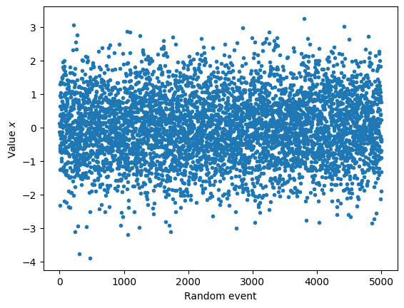
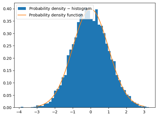
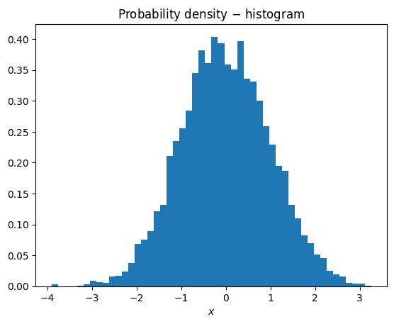
Below is also an example of the numerical generation of a normal distribution and a comparison with the theoretical probability density function.

Show code cell source

Hide code cell source

import numpy as np
import matplotlib.pyplot as plt

import sympy as sym
σ, μ, x, = sym.symbols('\\sigma, \\mu, x', real=True, positive=True)
π = sym.pi

p = 1/(σ*sym.sqrt(2*π)) * sym.exp(-(x-μ)**2/(2*σ**2))
data = {σ: 1., μ: 0.}
pdf = sym.lambdify(x, p.subs(data))


rng = np.random.default_rng(0)
x = rng.normal(loc=data[μ], scale=data[σ], size=5000)
#x = rng.uniform(low=-1, high=1, size=5000) # uniform distribution
plt.plot(x, '.')
plt.xlabel('Random event')
plt.ylabel('Value $x$')
plt.show()

plt.hist(x, bins=50, density=True, label='Probability density $-$ histogram')

x = np.linspace(-3*data[σ],3*data[σ], 100)
plt.plot(x, pdf(x), label='Probability density function')
plt.legend()
plt.show()

Central limit theorem

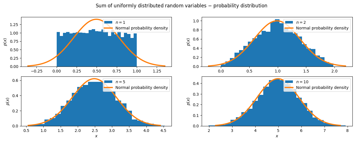
The central limit theorem states that the sum of independent random variables follows a normal distribution (regardless of the distribution of the original variables), provided that the sample size is sufficient.

The code below demonstrates the central limit theorem (CLT) using uniformly distributed random variables. The code creates N = 10 samples, where each sample has k = 5000 random values that follow a uniform distribution between 0 and 1. It then computes the sum of the first n samples (n = 1, 2, 5, 10) and shows their probability distributions with histograms. For each histogram, the theoretical normal distribution is also computed using the mean and standard deviation of the sum of n samples. It turns out that the sum of uniformly distributed samples converges to a normal distribution.

Show code cell source

Hide code cell source

import numpy as np
import sympy as sym
import matplotlib.pyplot as plt

seed = 123
rng = np.random.default_rng(seed)
N = 10 # number of random samples
k = 5000 # number of random values in a sample
data = [rng.uniform(low=0, high=1, size=k) for i in range(N)]

# summation for n = 1, 2, 5 and 10
S1 = np.sum(data[:1], axis=0) # n = 1
S2 = np.sum(data[:2], axis=0) # n = 2
S5 = np.sum(data[:5], axis=0) # n = 5
S10 = np.sum(data[:10], axis=0) # n = 10

σ, μ, x, = sym.symbols('\\sigma, \\mu, x', real=True, positive=True)
π = sym.pi
p = 1/(σ*sym.sqrt(2*π)) * sym.exp(-(x-μ)**2/(2*σ**2)) # theoretical probability density

fig, axs = plt.subplots(2, 2, figsize=(15, 5))
fig.suptitle(r'Sum of uniformly distributed random variables $-$ probability distribution')
bins = 25 # number of bins for the histogram

# plot for n = 1
axs[0, 0].hist(S1, bins=bins, density=True, label='$n=1$')
data = {σ: np.std(S1), μ: np.mean(S1)}
pdf = sym.lambdify(x, p.subs(data))
x_S1 = np.linspace(-3*data[σ]+data[μ], 3*data[σ]+data[μ], 100)
axs[0, 0].plot(x_S1, pdf(x_S1), lw=3, label='Normal probability density')
axs[0, 0].set_ylabel('$p(x)$')
axs[0, 0].legend(loc='upper right')

# plot for n = 2
axs[0, 1].hist(S2, bins=bins, density=True, label='$n=2$')
data = {σ: np.std(S2), μ: np.mean(S2)}
pdf = sym.lambdify(x, p.subs(data))
x_S2 = np.linspace(-3*data[σ]+data[μ], 3*data[σ]+data[μ], 100)
axs[0, 1].plot(x_S2, pdf(x_S2), lw=3, label='Normal probability density')
axs[0, 1].set_ylabel('$p(x)$')
axs[0, 1].legend(loc='upper right')

# plot for n = 5
axs[1, 0].hist(S5, bins=bins, density=True, label='$n=5$')
data = {σ: np.std(S5), μ: np.mean(S5)}
pdf = sym.lambdify(x, p.subs(data))
x_S5 = np.linspace(-3*data[σ]+data[μ],3*data[σ]+data[μ], 100)
axs[1,0].plot(x_S5, pdf(x_S5), lw=3, label='Normal probability density')
axs[1,0].set_xlabel('$x$')
axs[1,0].set_ylabel('$p(x)$')
axs[1,0].legend(loc='upper right')

# plot for n = 10
axs[1,1].hist(S10, bins=bins, density=True, label='$n=10$');
data = {σ: np.std(S10), μ: np.mean(S10)}
pdf = sym.lambdify(x, p.subs(data))
x_S10 = np.linspace(-3*data[σ]+data[μ],3*data[σ]+data[μ], 100)
axs[1,1].plot(x_S10, pdf(x_S10), lw=3, label='Normal probability density')
axs[1,1].set_xlabel('$x$')
axs[1,1].set_ylabel('$p(x)$')
axs[1,1].legend(loc='upper right');
plt.show()

The central limit theorem also states that the distribution of the sample of means of each random variable approaches the normal distribution as the sample size increases, even if the original population is distributed differently from normal. This holds if the samples are independent and identically distributed and the sample size is sufficient.

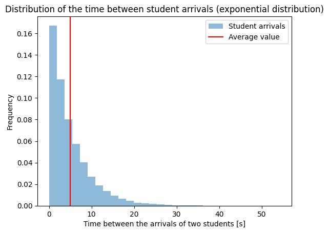
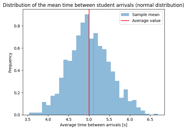
Let us now look at an example with a different distribution: we will track the exponentially distributed time between the arrivals of two students into a classroom. In the code below we create a very large sample: number_of_students = 100000 and observe that most students arrive with a time difference of less than 20 s. The next figure shows the sample means, where we divided the initial data into samples of size: sample_size = 100. We observe that the means are normally distributed.

Show code cell source

Hide code cell source

import numpy as np
import matplotlib.pyplot as plt

rate = 0.2
number_of_students = 100000

student_arrivals = np.random.exponential(scale=1/rate, size=number_of_students)

plt.hist(student_arrivals, bins=30, density=True, alpha=0.5, label='Student arrivals')
plt.xlabel('Time between the arrivals of two students [s]')
plt.ylabel('Frequency')
plt.title('Distribution of the time between student arrivals (exponential distribution)')
plt.axvline(x=1/rate, color='r', label='Average value')
plt.legend()
plt.show()


sample_size = 100
sample_means = np.mean(student_arrivals.reshape((sample_size,-1)),axis=0)

plt.hist(sample_means, bins=30, density=True, alpha=0.5, label='Sample mean')
plt.xlabel('Average time between arrivals [s]')
plt.ylabel('Frequency')
plt.title('Distribution of the mean time between student arrivals (normal distribution)')
plt.axvline(x=1/rate, color='r', label='Average value')
plt.legend()
plt.show()

Moments of the probability density function

In what follows, we will look at the tools for describing the properties of random processes. Let us assume that we have two random processes \(\left\{x_k(t)\right\}\) and \(\left\{y_k(t)\right\}\), where \(k\) is the index of the repetition of the process at time \(t\). We denote the statistical average of the entire ensemble of process repetitions (over the index \(k\)) as \(E[]\) (\(E[]\) denotes the expected value/generalized average; see also the link):

\[\begin{split} \begin{split} \mu_x(t) &= E[x(t)],\\ \mu_y(t) &= E[y(t)].\\ \end{split} \end{split}\]

Note: the above notation means that the average can change with time \(t\).

Note

We generalize the above expression by defining the \(\boldsymbol{n}\)-th moment of the probability density function:

\[ \mu_{x}^n(t)= E[x^n(t)] = \int_{-\infty}^{+\infty} x^n\, p(x)\, \textrm{d} x. \]

Covariance functions for two processes \(\left\{x_k(t)\right\}\) and \(\left\{y_k(t) \right\}\) are defined as:

\[\begin{split} \begin{split} C_{xx}(t, t+\tau) &= E \big[(x(t) - \mu_x(t)) \, (x(t+\tau) - \mu_x(t+ \tau))\big], \\ C_{yy}(t, t+\tau) &= E \big[(y(t) - \mu_y(t)) \, (y(t+\tau) - \mu_y(t+ \tau))\big], \\ C_{xy}(t, t+\tau) &= E \big[(x(t) - \mu_x(t)) \, (y(t+\tau) - \mu_y(t+ \tau))\big]. \\ \end{split} \end{split}\]

A special case worth attention is at \(\tau = 0\):

\[\begin{split} \begin{split} C_{xx}(t, t) &= E \big[(x(t) - \mu_x(t))^2\big]= \sigma_x^2(t), \\ C_{yy}(t, t) &= E \big[(y(t) - \mu_y(t))^2\big]= \sigma_y^2(t), \\ C_{xy}(t, t) &= E \big[(x(t) - \mu_x(t)) \, (y(t) - \mu_y(t))\big] = C_{xy}(t).\\ \end{split} \end{split}\]

The variances \(\sigma_x^2(t)\) and \(\sigma_y^2(t)\) are thus defined, and \(C_{xy}(t)\) is the covariance between \(\left \{x_k(t)\right\}\) and \(\left\{y_k(t)\right\}\) at time \(t\).

If we were to analyze a process with a two-dimensional normal distribution, the properties \(\sigma_x^2(t)\), \(\sigma_y^2(t)\) and \(C_{xy}(t)\) would be sufficient to describe the probability at particular time points \(t\).

Note

We generalize the above expression by defining the \(\boldsymbol{n}\)-th central moment of the probability density function:

\[ \sigma^n(t)= E[(x(t)-\mu_x)^n] = \int_{-\infty}^{+\infty} (x-\mu_x)^n\, p(x)\, \textrm{d} x. \]

Note

We say that two random processes \(\left\{x_k(t)\right\}\) and \(\left\{y_k(t)\right\}\) are weakly stationary when the mean values and covariance functions are time-independent. The processes are considered strongly stationary when the higher-order statistical moments and the cross moments are also time-independent. Since the Gaussian process is defined by two statistical moments (the probability distribution function can be derived solely from the mean values and covariances [Newland, 2012]), weak and strong stationarity coincide here.

Note

The autocorrelation function \(R_{xx}(\tau)\) and the cross-correlation function \(R_{xy}(\tau)\) are used for stationary random processes and are equal to the covariance functions in the case of a process with zero mean value:

\[\begin{split} \begin{split} R_{xx}(\tau) &= E[ x_k(t) \, x_k(t+\tau)], \\ R_{yy}(\tau) &= E[ y_k(t) \, y_k(t+\tau)], \\ R_{xy}(\tau) &= E[ x_k(t) \, y_k(t+\tau)]. \\ \end{split} \end{split}\]

Ergodicity

In an ergodic process, the statistical properties (e.g. the mean or the variance) can be determined, instead of over the ensemble of observations (\(k\)), on the basis of the time evolution (\(t\)) of a single observation.

Above (Moments of the probability density function), we determined the mean value over the ensemble of events. Assuming ergodicity, however, we can determine it on the basis of the time average:

\[\begin{split} \begin{split} \mu_x(k) &= \lim_{T \to \infty} \frac{1}{T}\int_{0}^{T} x_k(t)\, \textrm{d} t, \\ \mu_y(k) &= \lim_{T \to \infty} \frac{1}{T} \int_{0}^{T} y_k(t)\, \textrm{d} t.\\ \end{split} \end{split}\]

Simply put: if 1000 people simultaneously rolled a die in a game of Ludo, we would get a very similar result as if one person rolled the die 1000 times. Here we must assume that successive events in time (when one person is rolling) are not related to each other (e.g. that the die does not wear out over time). In the above equation we therefore observe the \(k\)-th process in time.

We can make a similar claim for the covariance function:

\[\begin{split} \begin{split} C_{xx}(\tau, k) &= \lim_{T \to \infty} \frac{1}{T} \int_{0}^{T} \left[x_k(t)-\mu_x(k)\right] \, \left[x_k(t+\tau) - \mu_x(k)\right] \textrm{d} t \\ &= R_{xx}(\tau, k) - \mu_x^2(k), \\ C_{yy}(\tau, k) &= \lim_{T \to \infty} \frac{1}{T} \int_{0}^{T} \left[y_k(t)-\mu_y(k)\right] \, \left[y_k(t+\tau) - \mu_y(k)\right] \textrm{d} t \\ &= R_{yy}(\tau, k) - \mu_y^2(k), \\ C_{xy}(\tau, k) &= \lim_{T \to \infty} \frac{1}{T} \int_{0}^{T} \left[x_k(t)-\mu_x(k)\right] \, \left[y_k(t+\tau) - \mu_y(k)\right] \textrm{d} t \\ &= R_{xy}(\tau, k) - \mu_x(k) \, \mu_y(k). \\ \end{split} \end{split}\]

Note

We say that a process is weakly ergodic if the time averages are equal to the averages of the ensemble of events, independently of the chosen \(k\):

\[\begin{split} \begin{split} \mu_x(k) &= \mu_x, \\ \mu_y(k) &= \mu_y, \\ C_{xx}(\tau, k) &= C_{xx}(\tau), \\ C_{yy}(\tau, k) &= C_{yy}(\tau), \\ C_{xy}(\tau, k) &= C_{xy}(\tau). \\ \end{split} \end{split}\]

If the conditions of weak ergodicity hold for all higher-order statistical properties, the process is strongly ergodic. For the Gaussian distribution, however, strong and weak ergodicity are interchangeable terms, as was the case with stationarity \(-\) the first moment and the second central moment are sufficient for a unique description of the Gaussian distribution. In such cases, the statistical properties of each separate sample function are representative of the entire ensemble. In the further analysis of ergodic processes we can therefore omit the index \(k\) and denote the sample function that fully describes the properties of the random process by \(x(t)\).

Ergodicity is important for various reasons: it simplifies the further theoretical treatment of random processes; even more importantly, it enables the analysis of actually measured random data. Instead of analyzing a large ensemble of time histories at the same time \(t\), it usually suffices to look at a single time history and, on the basis of the ergodicity assumption, extract the necessary statistical properties from it.

In structural dynamics we usually assume that the process has a zero mean, and therefore the variance \(\sigma_x^2\) can be computed in various ways:

\[\begin{split} \begin{split} \sigma_x^2 &= E \left[x^2(t)\right] = \int_{-\infty}^{+\infty} x^2 \, p(x)\, \textrm{d} x \\ &= \lim_{T \to \infty} \frac{1}{T} \int_{0}^{T} x^2(t)\,\textrm{d} t \\ &= \int_{-\infty}^{+\infty} S_{xx}(f)\,\textrm{d} f. \\ \end{split} \end{split}\]

In the above expressions it is assumed that \(x(t)\) represents periodic data with period \(T\). By \(S_{xx}(f)\) we denoted the power spectral density, and in this line we relied on Parseval’s theorem (see the chapter Parseval’s theorem and the power spectrum). We will look at the power spectral density in more detail in the next chapter. Note: if we consider a normally distributed process with zero mean value, the variance is the only missing parameter that uniquely determines such a distribution.

Power spectral density (PSD)

The power spectral density describes the frequency density of the power of a random process and complements the probability density function (\(p(x)\)) in the definition of a particular random process; the same probability density can have very different power spectral densities (PSD) in the frequency domain. We usually obtain the PSD with the Fourier transform, typically using the FFT algorithm.

The definition of the PSD is based on the autocorrelation function \(R_{xx}(\tau)\), which implicitly contains the frequency content of \(x(t)\) and at the same time satisfies the Dirichlet condition (at least in the case of processes with zero mean value):

\[ \int_{-\infty}^{+\infty} \left|x(t)\right| \textrm{d} t < \infty. \]

Since the autocorrelation function and the PSD are a Fourier transform pair, we can write the following (Wiener-Khinchin) relations for two random processes \(x(t)\) and \(y(t)\):

\[\begin{split} \begin{split} S_{xx}(f) &= \mathcal{F}\{R_{xx}(\tau)\}, \\ S_{yy}(f) &= \mathcal{F}\{R_{yy}(\tau)\}, \\ S_{xy}(f) &= \mathcal{F}\{R_{xy}(\tau)\}. \end{split} \end{split}\]

\(S_{xx}(f)\) and \(S_{yy}(f)\) (the PSD, also called the auto-spectral density) are even functions with positive real values. The cross-spectral density (also CSD) \(S_{xy}(f)\) generally has complex values.

Let us first look at the auto-spectral density:

\[\begin{split} \begin{split} S_{xx}(f) &= \int_{-\infty}^{+\infty} R_{xx}(\tau)\,\mathrm{e}^{-\mathrm{i}\,2\pi\,f\,\tau}\mathrm{d}\tau\\ &= \int_{-\infty}^{+\infty} \int_{-\infty}^{+\infty} x(t)\,x(t+\tau)\,\mathrm{e}^{-\mathrm{i}\,2\pi\,f\,\tau}\mathrm{d}t\,\mathrm{d}\tau;\qquad{\textrm{(substitute: }}t_1=t+\tau\textrm{)}\\ &= \int_{-\infty}^{+\infty} x(t)\,\,\mathrm{e}^{\mathrm{i}\,2\pi\,f\,t}\mathrm{d}t\,\int_{-\infty}^{+\infty} x(t_1)\,\mathrm{e}^{-\mathrm{i}\,2\pi\,f\,t_1}\,\mathrm{d}t_1\\ &=X^*(f)\,X(f). \end{split} \end{split}\]

In a similar way we could derive the cross-spectral density \(S_{xy}\).

In the case of real measurements, the time history is of finite length and the Dirichlet condition is satisfied; from the Fourier transform of the \(k\)-th time history:

\[\begin{split} \begin{split} X_k(f, T) &= \int_0^T x_k(t) \,\mathrm{e}^{- \textrm{i} \, 2 \pi \, f \, t} \,\textrm{d} t, \\ Y_k(f, T) &= \int_0^T y_k(t) \,\mathrm{e}^{- \textrm{i} \, 2 \pi \, f \, t} \,\textrm{d} t \\ \end{split} \end{split}\]

we can, by multiplying the Fourier transforms, determine the cross-spectral density (since we have a finite-length signal, to obtain a density we must normalize by \(T\)):

\[ S_{xy}(f, T, k) = \frac{1}{T}\, X_k^*(f, T) \, Y_k(f, T). \]

Note

The auto- (PSD) and cross-spectral (CSD) power spectral density are therefore defined, for the case of an ergodic process, as (without the index \(k\)):

\[\begin{split} \begin{split} S_{xx}(f) &= \frac{1}{T}\, X^*(f) \, X(f)\qquad\text{PSD},\\ S_{xy}(f) &= \frac{1}{T}\, X^*(f) \, Y(f)\qquad\text{CSD}. \end{split} \end{split}\]

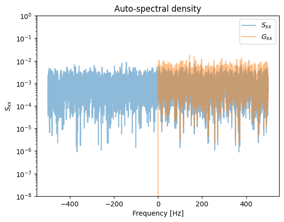
The auto-spectral density \(S_{xx}(f)\) covers negative and positive frequencies and is therefore also called the two-sided spectral density function. Often the one-sided spectral density function \(G_{xx}(f)\) is used, which is defined as:

\[\begin{split} G_{xx}(f) = \begin{cases} 2\,S_{xx}(f),& f>0,\\ S_{xx}(f),& f=0,\\ 0,& f<0. \end{cases} \end{split}\]

The same holds for \(G_{xy}(f)\). For the two-sided cross-spectral density, \(S_{xy}(f)=S_{yx}^*(f)\).

Example 1

Let us first look at the computation of the auto-spectral density with the help of the Fourier transform. At the end of the example we verify Parseval’s theorem in discrete form:

\[ \sigma_x^2 = \frac{1}{T} \int x^2(t)\,\textrm{d} t = \int S_{xx}(f)\,\textrm{d} f. \]

In this example, be careful about how \(S_{xx}(f)\) and \(G_{xx}(f)\) are treated.

Show code cell source

Hide code cell source

import numpy as np
from scipy.signal import welch 
import matplotlib.pyplot as plt

rng = np.random.default_rng(0)
N = 5000
fs = 1000
dt = 1./fs
x = rng.normal(size=N)
time = np.arange(N)*dt
T = dt*N
plt.plot(time, x, '.')
plt.xlabel('Time [t]')
plt.ylabel('Value $x$')
plt.show()

plt.title('Probability density $-$ histogram')
plt.xlabel('$x$')
plt.hist(x, bins=50, density=True)
plt.show()

X = np.fft.fft(x)/N
freq = np.fft.fftfreq(N, d=dt)
scale = 1.0 * N / fs # scaling to density
Sxx = X.conj()*X * scale

X_r = np.fft.rfft(x)/N
freq_r = np.fft.rfftfreq(N, d=dt)
Gxx = 2*X_r.conj()*X_r * scale

# alternative computation via SciPy (this is actually how it is done later)
freq2, Gxx2 = welch(x, window=np.ones_like(x), fs=fs)

plt.title('Auto-spectral density')
plt.semilogy(freq, np.abs(Sxx), alpha=0.5, label='$S_{xx}$')
plt.semilogy(freq2, np.abs(Gxx2), alpha=0.5, label='$G_{xx}$')
plt.ylim(1e-8,1e0)
plt.legend()
plt.xlabel('Frequency [Hz]')
plt.ylabel('$S_{xx}$')
plt.show()

print('Integral in time: ', np.trapezoid(x*x, dx=dt)/(N/fs), 
      '\nIntegral PSD (Sxx): ', np.trapezoid(np.real(Sxx), dx=1/(N/fs)), 
      '\nIntegral PSD (Gxx): ', np.trapezoid(np.real(Gxx), dx=1/(N/fs)),
      '\nIntegral PSD (Gxx) Welch: ', np.trapezoid(np.real(Gxx2), dx=1/(N/fs)))

Integral in time:  0.9904720416233659 
Integral PSD (Sxx):  0.990606212416766 
Integral PSD (Gxx):  0.9908307702229944 
Integral PSD (Gxx) Welch:  0.9907922407740424

We can also look at the computation of the variance with the built-in numpy.var() method:

np.var(x)

np.float64(0.9908102289544899)

Small differences arise because in our code we assumed (np.var does not make this assumption) that the time series x has a mean value of zero, which, however, is not entirely true:

np.mean(x)

np.float64(-0.004532247621656686)

Example 2

Let us now look at an example and first compute the variance with the help of the definition of the normal distribution with zero mean value \(\mu=0\) and standard deviation \(\sigma=3\):

\[ \sigma_x^2 = E \left[x^2(t)\right] = \int_{-\infty}^{+\infty} x^2 \, p(x)\, \textrm{d} x. \]

import sympy as sym
σ, μ, x, = sym.symbols('\\sigma, \\mu, x', real=True, positive=True)
π = sym.pi

p = 1/(σ*sym.sqrt(2*π)) * sym.exp(-(x-μ)**2/(2*σ**2))

data = {σ: 3., μ: 0.}

sym.integrate(x**2*p, (x, -sym.oo, +sym.oo)).subs(data)

\[\displaystyle 9.0\]

We obtained the expected value \(\sigma^2=9\). We continue with the integration of the time series in time:

\[ \sigma_x^2 = \lim_{T \to \infty} \frac{1}{T} \int_{0}^{T} x^2(t)\,\textrm{d} t. \]

import numpy as np

σ = 3
rng = np.random.default_rng(0)
N = 1_000_000
T = 10
time,  dt = np.linspace(0, T, N, retstep=True)
fs = 1/dt
x = rng.normal(scale=σ, size=N)

np.trapezoid(x**2, dx=dt)/T

np.float64(9.012114810596122)

Since this is numerical data, we obtained a value that is more or less close to the expected value \(\sigma^2=9\) (try changing N). We continue with the computation of the variance in the frequency domain:

\[ \sigma_x^2 = \int_{-\infty}^{+\infty} S_{xx}(f)\,\textrm{d} f. \]

Or using the one-sided amplitude spectrum:

X = np.fft.fft(x)/N  # scaling to amplitude
df = fs/N
scale = 1/df     # scaling to density (frequency axis)
Sxx = np.real(X.conj()*X) * scale
np.sum(Sxx)/scale

np.float64(9.012106104865358)

X_r = np.fft.rfft(x)/N
df = fs/N
scale = 1/df
Gxx = np.real(X_r.conj()*X_r) * scale
Gxx[1:] = 2*Gxx[1:]
np.sum(Gxx)/scale

np.float64(9.012110027353884)

Spectral moments

From the definition of the PSD it follows that the area under the curve is equal to the expected squared value \(E[x^2]\) of the process (see the chapter Parseval’s theorem and the power spectrum):

\[ m_0 = E \left[x^2(t)\right] = \int_{-\infty}^{+\infty} S_{xx}(\omega)\, \textrm{d} \omega, \]

where \(m_0\), the zeroth spectral moment, is equal to the variance \(\sigma_x^2\) of a process with zero mean value. The higher even moments correspond to the variance of the time derivatives of the original random process:

\[ m_2 = E \left[\dot{x}^2(t)\right] = \int_{-\infty}^{+\infty} \omega^2 \, S_{xx}(\omega) \,\textrm{d} \omega. \]

The general expression for the \(i\)-th spectral moment \(m_i\) can be written in the form:

\[ m_i = \int_{-\infty}^{+\infty} \omega^i \, S_{xx}(\omega) \textrm{d} \omega=\int_{0}^{+\infty} \omega ^i \, G_{xx}(\omega) \,\textrm{d} \omega, \]

where \(G_{xx}\) is the one-sided PSD.

It must be emphasized that \(-\) if the PSD is given in Hz (\(G_{xx}(f)\)) \(-\) we must be careful about the correct use of the factor \((2\pi\,f)^i\):

\[ m_i = \int_{0}^{+\infty} (2\pi\,f)^i \, G_{xx}(f) \,\textrm{d} f. \]

Example

Let us again look at an example; first let us define a harmonic response with amplitude \(A=1\). The variance of the displacement is expected to be: \((A/\sqrt{2})^2=0.5\,A\), the variance of the velocity: \(((2\pi\,f_0\,A)/\sqrt{2})^2=2\pi^2\,f_0^2\,A\) and the variance of the acceleration: \((((2\pi\,f_0)^2\,A)/\sqrt{2})^2=2^3(\pi\,f_0)^4\,A\).

Show code cell source

Hide code cell source

import numpy as np
import matplotlib.pyplot as plt

N = 1_000_000
T = 10
f_0 = 100
time,  dt = np.linspace(0, T, N, retstep=True)
x = np.sin(2*np.pi*f_0*time)
X = np.fft.rfft(x)/N
freq = np.fft.rfftfreq(N, dt)

plt.title('First 5000 points of the deterministic signal')
plt.plot(time[:5000], x[:5000])
plt.xlabel('$t$ [s]')
plt.ylabel('$x$')

np.trapezoid(x**2, dx=dt)/T

np.float64(0.5)

Let us define a function for the spectral moments:

def spectral_moment(X_r, freq, i=0):
    # we do not use scale here, since it cancels out
    Gxx = X_r.conj()*X_r
    Gxx[1:] = 2*Gxx[1:]
    return np.real(np.sum((2*np.pi*freq)**i * Gxx))

Spectral moment \(m_0\) (displacement): let us verify that we indeed obtain the expected value (\(0.5\,A=0.5\)) in the frequency domain as well:

spectral_moment(X_r=X, freq=freq, i=0)

np.float64(0.4999995)

Spectral moment \(m_2\) (velocity): for the velocity we expect the value \(2\,\pi^2\,f_0^2\,A=197392.08\):

spectral_moment(X_r=X, freq=freq, i=2)

np.float64(197392.0431335743)

Or in time:

v = np.gradient(x)/dt
np.trapezoid(v**2, dx=dt)/T

np.float64(197389.49045450424)

Spectral moment \(m_4\) (acceleration): for the acceleration we expect \(2^3(\pi\,f_0)^4\,A=77927272827.2\):

spectral_moment(X_r=X, freq=freq, i=4)

np.float64(100537876580.76273)

Or in time:

a = np.gradient(v)/dt
np.trapezoid(a**2, dx=dt)/T

np.float64(77925221885.31584)

We already observe a relatively large deviation; the reason is numerical error. The amplitude spectrum \(X\) has, outside \(f_0\), a theoretical value of 0, but an actual value close to 0; since the expression for computing the fourth spectral moment strongly emphasizes high frequencies (\((2\pi\,f)^4\)), the numerical error is also emphasized. We obtain a better result if, for example, we limit ourselves in frequency:

sel = np.logical_and(freq>=(f_0-1),freq<=(f_0+1))
spectral_moment(X_r=X[sel], freq=freq[sel], i=4)

np.float64(77926867176.11658)