5. Data quantization

Uniform time sampling

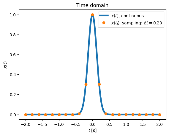
So far we have dealt with continuous data \(x(t)\), but in experimental work we almost always encounter discrete values, which are typically captured by uniform time sampling \(x(n\,\Delta t)\), where \(\Delta t\) is the sampling time (period) (\(f_s=1/\Delta t\) is the sampling frequency).

In understanding sampled data, we help ourselves with uniformly sampled data \(x_s(t)\), which are the product of the continuous data \(x(t)\) and a train of impulses \(i(t)\):

\[ x_s(t)=x(t)\,i(t), \]

where:

\[ i(t)= \sum_{n=-\infty}^{+\infty}\delta(t-n\,\Delta t). \]

The Fourier transform of \(x_s(t)\) is:

\[\begin{split} \begin{split} X_s(f)&=\int_{-\infty}^{+\infty} x(t)\,\sum_{n=-\infty}^{+\infty}\delta(t-n\,\Delta t)\,\mathrm{e}^{-\textrm{i}\,2\pi\,f\,t}\,\textrm{d} t\\ &=\sum_{n=-\infty}^{+\infty}\,\int_{-\infty}^{+\infty} x(t)\,\mathrm{e}^{-\textrm{i}\,2\pi\,f\,t}\,\delta(t-n\,\Delta t)\,\textrm{d} t\\ &=\sum_{n=-\infty}^{+\infty}\,x(n\,\Delta t)\,\mathrm{e}^{-\textrm{i}\,2\pi\,f\,n\,\Delta t}. \end{split} \end{split}\]

In the transition to the last line, we use the sifting property of the Dirac delta function (see the chapter Properties of the Dirac delta function).

The key consequence of the above derivation is: for sampled data, the integral is transformed into a sum of sampled values (multiplied by a harmonic modulation).

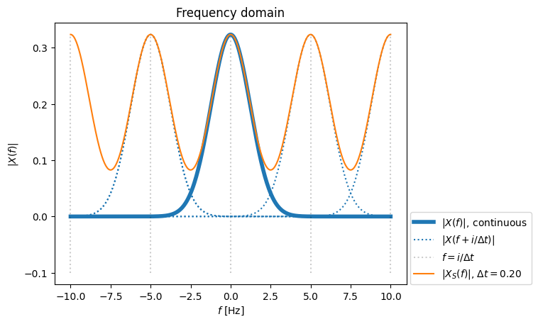
We also find that the Fourier transform of the uniformly sampled series \(X_s(f)\) repeats (is periodic) with frequency \(1/\Delta t\), which we prove as follows:

\[\begin{split} \begin{split} X_s(f+r/\Delta t)&=\sum_{n=-\infty}^{+\infty}\,x(n\,\Delta t)\,\mathrm{e}^{-\textrm{i}\,2\pi\,(f+r/\Delta t)\,n\,\Delta t}\\ &=\sum_{n=-\infty}^{+\infty}\,x(n\,\Delta t)\,\mathrm{e}^{-\textrm{i}\,2\pi\,f\,n\,\Delta t}\,\underbrace{\mathrm{e}^{-\textrm{i}\,2\pi\,r\,n}}_{=1}\\ &=\sum_{n=-\infty}^{+\infty}\,x(n\,\Delta t)\,\mathrm{e}^{-\textrm{i}\,2\pi\,f\,n\,\Delta t}\\ &=X_s(f), \end{split} \end{split}\]

where \(r\) is an arbitrary integer. We therefore conclude:

Note

The Fourier transform of data \(x(t)\), sampled with period \(\Delta t\), is defined as the sum:

\[ X_s(f)=\sum_{n=-\infty}^{+\infty}\,x(n\,\Delta t)\,\mathrm{e}^{-\textrm{i}\,2\pi\,f\,n\,\Delta t} \]

and is periodic in the frequency domain with frequency \(1/\Delta t\):

\[ X_s(f)=X_s(f+r/\Delta t), \qquad \textrm{where:}\quad r\in \mathbb{Z}. \]

Let us now try to derive the inverse Fourier transform; first we multiply the expression in the frequency domain by \(\mathrm{e}^{\textrm{i}\,2\pi\,f\,p\,\Delta t}\) (here \(p\,\Delta t\) is the time at which we are interested in the value in time \(x(p\,\Delta t)\)) and integrate over the frequency \(f\):

\[ \int_{-1/(2\Delta t)}^{+1/(2\Delta t)}\,X_s(f)\,\mathrm{e}^{\textrm{i}\,2\pi\,f\,p\,\Delta t}\,\textrm{d}f=\int_{-1/(2\Delta t)}^{+1/(2\Delta t)}\,\sum_{n=-\infty}^{+\infty}\,x(n\,\Delta t)\,\mathrm{e}^{-\textrm{i}\,2\pi\,f\,n\,\Delta t}\,\mathrm{e}^{\textrm{i}\,2\pi\,f\,p\,\Delta t}\,\textrm{d}f, \]

where we integrated only over one period in frequency (it would not make sense to integrate over more, since \(X_s(f)\) is a periodic function).

We rewrite the above expression into:

\[ \sum_{n=-\infty}^{+\infty}\,x(n\,\Delta t)\,\int_{-1/(2\Delta t)}^{+1/(2\Delta t)}\,\underbrace{\mathrm{e}^{-\textrm{i}\,2\pi\,f\,(n-p)\,\Delta t}}_{=1,\textrm{ when } n = p;\quad\textrm{otherwise the integral of the expression is: }0}\,\textrm{d}f=x(p\,\Delta t)\,\frac{1}{\Delta t}. \]

Note

We have thus derived the inverse Fourier transform:

\[ x(p\,\Delta t) = \Delta t\,\int_{-1/(2\Delta t)}^{+1/(2\Delta t)}\,X_s(f)\,\mathrm{e}^{\textrm{i}\,2\pi\,f\,p\,\Delta t}\,\textrm{d}f. \]

Aliasing

Aliasing (also frequency folding) is a phenomenon in which a frequency in the signal is identified incorrectly; the reason for this is inappropriate sampling of the time signal. Let us look at the details: the train of impulses \(i(t)\) can be treated as periodic data with period \(\Delta t\), and described by a Fourier series:

\[ i(t)= \sum_{n=-\infty}^{+\infty}\delta(t-n\,\Delta t) = \sum_{n=-\infty}^{+\infty}c_n\,\mathrm{e}^{\textrm{i}\,2\pi\,n\,t/\Delta t}, \]

where:

\[ c_n=\frac{1}{\Delta t}\,\int_{-\Delta t/2}^{+\Delta t/2}i(t)\,\mathrm{e}^{-\textrm{i}\,2\pi\,n\,t/\Delta t}\,\textrm{d}t=\frac{1}{\Delta t}. \]

It follows:

\[ i(t)= \frac{1}{\Delta t}\, \sum_{n=-\infty}^{+\infty}\mathrm{e}^{\textrm{i}\,2\pi\,n\,t/\Delta t}. \]

The Fourier transform of \(i(t)\), defined with the help of Fourier series:

\[\begin{split} \begin{split} I(f)&= \int_{-\infty}^{+\infty}\Big(\frac{1}{\Delta t}\, \sum_{n=-\infty}^{+\infty}\mathrm{e}^{\textrm{i}\,2\pi\,n\,t/\Delta t}\Big)\, \mathrm{e}^{-\textrm{i}\,2\pi\,f\,t}\,\textrm{d}t\\ &= \frac{1}{\Delta t}\, \sum_{n=-\infty}^{+\infty}\int_{-\infty}^{+\infty} \mathrm{e}^{\textrm{i}\,2\pi\,n\,t/\Delta t}\, \mathrm{e}^{-\textrm{i}\,2\pi\,f\,t}\,\textrm{d}t\\ &= \frac{1}{\Delta t}\, \sum_{n=-\infty}^{+\infty}\int_{-\infty}^{+\infty} \mathrm{e}^{-\textrm{i}\,2\pi\,(f-n/\Delta t)\,t}\,\textrm{d}t\\ &= \frac{1}{\Delta t}\, \sum_{n=-\infty}^{+\infty} \delta\Big(f-\frac{n}{\Delta t}\Big).\\ \end{split} \end{split}\]

Above, we used the property of the Dirac delta function \(\int_{-\infty}^{+\infty}\mathrm{e}^{\pm\textrm{i}\,2\pi\,a\,t}\,\textrm{d}t= \delta(a)\) (see the chapter Properties of the Dirac delta function). The Fourier transform of \(i(t)\) is therefore periodically repeating in the frequency domain with frequency period \(1/\Delta t\).

Let us now look at the relation between \(X(f)\) and \(X_s(f)\):

\[\begin{split} \begin{split} X_s(f) =\mathcal{F}\left\{i(t)\,x(t)\right\} &= I(f)*X(f)\\ &=\int_{-\infty}^{+\infty}I(p)\,X(f-p)\,\textrm{d}p\\ &=\int_{-\infty}^{+\infty}\frac{1}{\Delta t}\, \sum_{n=-\infty}^{+\infty} \delta\Big(p-\frac{n}{\Delta t}\Big)\,X(f-p)\,\textrm{d}p\\ &=\frac{1}{\Delta t}\,\sum_{n=-\infty}^{+\infty}\,\underbrace{\int_{-\infty}^{+\infty}\, \delta\Big(p-\frac{n}{\Delta t}\Big)\,X(f-p)\,\textrm{d}p}_{\textrm{Sifting property at $p=n/\Delta t$}}\\ &=\frac{1}{\Delta t}\,\sum_{n=-\infty}^{+\infty}\,X\Big(f-\frac{n}{\Delta t}\Big)\\ \end{split} \end{split}\]

How do we interpret the above derivation? If we have time-sampled data \(x_s(t)\), which in the frequency domain leads to \(X_s(f)\), then at a certain frequency \(f\) we have the content of the sum of the continuous data \(X(f)\) at the frequencies \(f-n/\Delta t\), where the integer \(n\) goes from \(-\infty\) to \(+\infty\). In practice this means that the content of the actual (continuous) signal from the frequency range outside the range \([-1/(2\Delta t), +1/(2\Delta t)]\) is folded and overlaps into the frequency range \([-1/(2\Delta t),\,+1/(2\Delta t)]\); see the example below.

Example: Gaussian impulse

Here we will look at time sampling and aliasing on the example of a Gaussian impulse/window (see the chapter Gaussian impulse), which is defined in the time and frequency domains as:

\[ x(t) = \mathrm{e}^{-a\,t^2},\quad X(f)=\sqrt{\frac{\pi}{a}}\, \mathrm{e}^{-\pi^{2}\,f^{2}/a};\qquad a>0. \]

Show code cell source

Hide code cell source

import sympy as sym
import matplotlib.pyplot as plt
import numpy as np

# instruction: vary the parameter `a`

t, f = sym.symbols('t, f', real=True)
n, Δt = sym.symbols('n, Δt')
a = sym.symbols('a', real=True, positive=True)
x = sym.exp(-a*t**2)
X = sym.fourier_transform(x, t, f)
Xsum = sym.Sum(X.subs(f, f-n/Δt), (n, -10, 10))

data = {a: 30, Δt: .2}
# prepare vectorized functions for numpy
f_x = sym.lambdify(t, x.subs(data), 'numpy')
f_X_abs = sym.lambdify(f, sym.Abs(X.subs(data)), 'numpy')
f_Xsum_abs = sym.lambdify(f, sym.Abs(Xsum.subs(data)), 'numpy')

# value ranges in time and frequency (t_g are 'dense' data for displaying the continuous function)
N = int(2/data[Δt]) # approximate number -N so that the time range is about [-2,2]
t_g = np.arange(-10*N,10*N+1)*data[Δt]/10
n = np.arange(-N,N+1)
t_i = n*data[Δt]
K = 2 # how many neighboring copies of X(f) we show
fr = np.linspace(-K/data[Δt],K/data[Δt], num=500)

plt.title('Time domain')
plt.plot(t_g, f_x(t_g), 'C0', label='$x(t)$, continuous', linewidth=4)
plt.plot(t_i, f_x(t_i), color='C1', marker='o', ls='', label=f'$x(t_i)$, sampling: $\\Delta t=${data[Δt]:3.2f}')
plt.xlabel('$t$ [s]')
plt.ylabel('$x(t)$')
plt.legend()
plt.show()

plt.title('Frequency domain')
plt.plot(fr, f_X_abs(fr), 'C0', label='$|X(f)|$, continuous', linewidth=4)
for i in range(-K,K):
    plt.plot(fr, f_X_abs(fr+i/data[Δt]), 'C0', ls=':')
    plt.vlines(i/data[Δt], -0.1, np.max(f_X_abs(fr)), 'k', ls=':', alpha=0.2)
plt.plot(fr, f_X_abs(fr+i/data[Δt]), 'C0', ls=':', label='$|X(f+i/\\Delta t)|$')
plt.vlines((i+1)/data[Δt], -0.1, np.max(f_X_abs(fr)), 'k', ls=':', alpha=0.2, label='$f=i/\\Delta t$')
plt.plot(fr, f_Xsum_abs(fr), color='C1', label=f'$|X_S(f)|$, $\\Delta t=${data[Δt]:3.2f}')
plt.xlabel('$f$ [Hz]')
plt.ylabel('$|X(f)|$')
plt.legend(loc=(1.01,0))
plt.show()

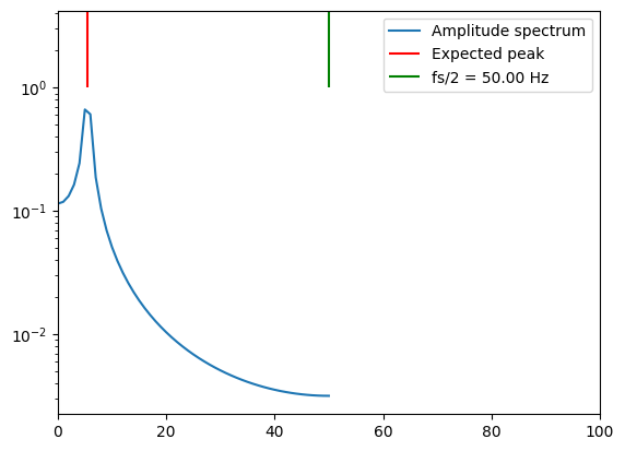
Another example of aliasing is the example below, where we consider harmonic data. When the sampling frequency fs is too low relative to the frequency of the harmonic data f (\(f>fs/2\)), the actual frequency is folded into the frequency range up to fs/2. In the code below, try slowly raising the frequency of the sine signal f toward (and above) the sampling frequency fs.

Show code cell source

Hide code cell source

import matplotlib.pyplot as plt
import numpy as np

f = 5.5 # <<<<<<<<<<<<<<<<
T = 1.
N = 100
t, dt = np.linspace(-T/2, T/2, N, endpoint=False, retstep=True)
fs = 1/dt
x = np.cos(2*f*np.pi*t+0.33)

X1=np.fft.rfft(x)*2/len(x)

f1=np.fft.rfftfreq(len(x),dt)
plt.semilogy(f1, np.abs(X1), label='Amplitude spectrum');
plt.vlines(f, 1, 1000, 'r', label='Expected peak')
plt.vlines(fs/2, 1, 1000, 'g', label=f'fs/2 = {fs/2:3.2f} Hz')
plt.xlim(0, fs/2+50)
plt.legend();

Preventing aliasing

If \(f_s=1/\Delta t\) is the sampling frequency, then aliasing can be avoided by using a low-pass filter at the frequency:

\[ f_{np}<\frac{f_s}{2}. \]

Here it is important to use an analog filter before performing the time sampling. The frequency \(f_{np}\) is also called the Nyquist frequency.

Data quantization: converting continuous data into discrete data

For computer processing, we must convert the measured continuous data into discrete numerical values, captured at a certain sampling frequency. Acquisition cards today allow relatively fast acquisition (at least 100 kHz) at a relatively large dynamic depth (at least 24 bits). Here we will look in more detail at the dynamic depth, which represents the number of discrete levels at which the acquisition card distinguishes the analog data.

The representation of numbers in a computer is of finite precision; today’s computers usually use 64-bit precision, which is significantly more precise than what acquisition measurement cards allow.

Let us look at the following example, where we consider a sinusoid. If we use a 24-bit card and the typical measurement range [-10, 10], the difference between two quantization levels is approximately 1e-6, which is entirely sufficient for most measurements. The ratio between the smallest and the largest value that we can measure on a particular acquisition card is called the dynamic range or also the dynamic depth.

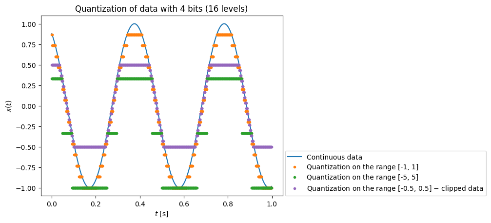
If, however, we use a system with a lower dynamic range, then we must pay very close attention to the measurement range in connection with the dynamic range, and possibly amplify the measured data. Such an example is the sinusoid below, which we quantize on two ranges ([-1, 1] and [-5, 5]) with 4-bit precision (16 levels).

When measuring, we must also watch out for clipped data (clipping), when the measurement range is too small (example below: [-0.5, 0.5]).

Note: the code for the figure below also includes an example where noise can help us measure quantities that are smaller than the quantization level.

Show code cell source

Hide code cell source

import matplotlib.pyplot as plt
import numpy as np

T = 1
N = 1000
fr = 2.452
t, dt = np.linspace(0, T, N, endpoint=False, retstep=True)
angle = 0.5
x = 1*np.cos(2*np.pi*fr*t+angle)
# This example shows how random noise can help us measure something that is below the quantization level.
#x = 0.03*np.cos(2*np.pi*fr*t+angle)
#x = x+.2*(np.random.rand(N)-0.5)

def get_quantized(x, bits = 4, adc_range = (-2, 2)):
    x2 = x.copy()
    lo, hi = adc_range
    x2[x<=lo] = lo
    x2[x>=hi] = hi
    delta = (hi - lo) / (2**(bits)-1)
    qnt = lo+delta*np.floor((x2-lo)/delta)
    return qnt

bits = 4
levels = 2**bits
x2 = get_quantized(x, bits = bits, adc_range=(-1, 1))
x3 = get_quantized(x, bits = bits, adc_range=(-5, 5))
x4 = get_quantized(x, bits = bits, adc_range=(-.5, .5))

plt.title(f'Quantization of data with {bits} bits ({levels} levels)')
plt.plot(t, x, 'C0', label='Continuous data')
plt.plot(t, x2, 'C1', marker='.', linestyle='', label=f'Quantization on the range [-1, 1]')
plt.plot(t, x3, 'C2', marker='.', linestyle='', label=f'Quantization on the range [-5, 5]')
plt.plot(t, x4, 'C4', marker='.', linestyle='', label=f'Quantization on the range [-0.5, 0.5] $-$ clipped data')
plt.xlabel('$t$ [s]')
plt.ylabel('$x(t)$')
plt.legend(loc=(1.01,0))
plt.show()

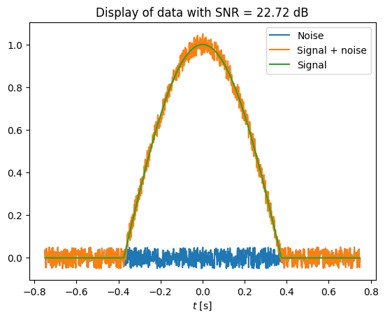
Signal-to-noise ratio

The difference between the quantized and the actual value can be treated as random noise \(e\) with a uniform distribution within the quantization step. The standard deviation of such noise is defined as (Shin and Hammond [2008], p.: 133):

\[ \sigma_e=\frac{A/2^b}{\sqrt{12}}, \]

where \(A\) is the total span of the quantization range and \(b\) the number of quantization bits, without the sign bit. For 24-bit quantization on the range from -10 to 10 (\(A=20\)), the standard deviation of the noise is:

\[ \sigma_e = \frac{20/2^{23}}{\sqrt{12}}=6.88\cdot 10^{-7}. \]

In evaluating the proportion of useful information relative to noise, we help ourselves with:

Note

the signal-to-noise ratio:

\[ \textrm{SNR}=10\log_{10}\Big(\frac{\sigma_x^2}{\sigma_e^2}\Big), \]

where \(\sigma_x^2\) and \(\sigma_e^2\) represent the power of the useful information (the signal \(x\)) and of the noise (\(e\)).

If we assume that \(\sigma_x=A/4\) (to prevent clipping of the data), we derive:

\[ \textrm{SNR}=10\log_{10}\Big(\frac{(A/4)^2}{\big(\frac{A/2^b}{\sqrt{12}}\big)^2}\Big)= 10\log_{10}\big(3/4\cdot 2^{2b}\big)\approx -1.25+6\,b\,\textrm{dB}. \]

In the case of 12-bit quantization, \(b=11\) and we have approximately 65 dB of dynamic range available, while in the case of 24-bit quantization the range would theoretically be approximately 137 dB. In practice we also deal with other sources of noise, which cause the SNR values to be significantly lower. Below, an idealized example of noise and of data not burdened with noise is shown.

Show code cell source

Hide code cell source

import sympy as sym
import matplotlib.pyplot as plt
import numpy as np

T = 1.5
N = 1000
w = 0.5
t = np.linspace(-T/2, T/2, N, endpoint=False)
dt = t[1] - t[0]
x = np.cos(2*np.pi*t/(2*w*T))
x[np.logical_or(-w*T*0.5 > t , t > w*T*0.5)] = 0.
n = 0.1*(np.random.rand(N)-0.5)

plt.title(f'Display of data with SNR = {10*np.log10(np.std(x)**2/np.std(n)**2):3.2f} dB')
plt.plot(t, n, label='Noise')
plt.plot(t, x+n, label='Signal + noise')
plt.plot(t, x, label='Signal')
plt.xlabel('$t$ [s]')
plt.legend()
plt.show()