4. Linear time-invariant systems with one degree of freedom

A single-degree-of-freedom system (SDOF, figure below) can be described by an inhomogeneous second-order ordinary differential equation:

\[ m\,\ddot{x}(t)+c\,\dot{x}(t)+k\,x(t)=f(t), \]

where \(f(t)\) is the excitation force. The solution of the inhomogeneous equation is of the form:

\[ x(t) = x_{h}(t) + x_{p}(t), \]

where \(x_{h}\) is the homogeneous solution and \(x_{p}\) the particular solution.

Free response (homogeneous solution)

If there is no excitation force, \(f(t)=0\), the homogeneous solution is obtained from:

\[ m\,\ddot{x}_{h}(t)+c\,\dot{x}_{h}(t)+k\,x_{h}(t)=0. \]

We use the ansatz for the solution \(x_{h}(t)\):

\[ x_{h}(t)=X_{h}\,\mathrm{e}^{\lambda \,t}, \]

where the displacement amplitude \(X_{h}\) and the eigenvalue \(\lambda\) are unknown (and must be determined). We insert the ansatz into the differential equation:

\[ \lambda^2\,m\,X_{h}\,\mathrm{e}^{\lambda \,t}+\lambda\,c\,X_{h}\,\mathrm{e}^{\lambda \,t}+k\,X_{h}\,\mathrm{e}^{\lambda \,t}=0. \]

We rearrange the expression:

\[ \left(\lambda^2\,m+\lambda\,c+k\right)\,X_{h}\,\mathrm{e}^{\lambda \,t}=0. \]

We determine the nontrivial (\(X_{h}\,\mathrm{e}^{\lambda \,t}\neq0\)) solution on the basis of the characteristic equation:

\[ \lambda^2\,m+\lambda\,c+k=0. \]

The solution of the characteristic equation is:

\[ \lambda_{1,2}=-\frac{c}{2\,m} \pm \frac{\sqrt{c^2-4\,k\,m}}{2\,m}, \]

where \(\lambda_{1,2}\) are the eigenvalues of the system (in general a complex number).

Depending on the ratio between the inertial, elastic and damping forces, the solution is:

• overdamped: if the damping forces dominate over the inertial and elastic forces (\(c^2\geq 4\,k\,m\)),

• critically damped: if the damping forces are equal to the inertial and elastic forces (\(c^2=4\,k\,m\)),

• underdamped: if the inertial and elastic forces dominate over the damping forces (\(c^2\leq 4\,k\,m\)).

In the case of an overdamped and a critically damped system, the solution is in real form and the motion is not oscillatory.

In this book we focus on the underdamped case, when the complex eigenvalues are conjugate pairs. The mass \(m\), the damping \(c\) and the stiffness \(k\) define the undamped natural angular frequency (also resonant frequency, natural frequency):

\[ \omega_0 = \sqrt{\frac{k}{m}}. \]

Here it is important to recall (see the basic courses on dynamics and mechanical vibrations) that in linear systems a preload does not change the natural frequency.

Damping can be defined with the help of the damping ratio:

\[ \delta = \frac{c}{c_{c}}, \]

where:

\[ c_{c} = 2\,\sqrt{k\,m} \]

is the critical damping.

With the help of the undamped natural frequency \(\omega_0\) and the damping ratio \(\delta\), we can rewrite the homogeneous differential equation into the standard form:

\[ \ddot{x}_{h}(t)+2\,\delta\,\omega_0\,\dot{x}_{h}(t)+\omega_0^2\,x_{h}(t) =0. \]

Furthermore, we insert \(\omega_0\) and \(\delta\) into the expression for the eigenvalues:

\[ \lambda_{1,2}=-\delta\, \omega_0 \pm \mathrm{i}\,\omega_{d}, \]

where:

\[ \omega_{d} = \omega_0\,\sqrt{1-\delta^2} \]

is called the damped natural angular frequency (it is correctly denoted by \(\omega_{0,d}\), but here, for the sake of the notation in the code below, we use the short form).

We insert the derived eigenvalues into the ansatz for the homogeneous solution \(x_{h}(t)\). Since we have two eigenvalues, the general solution is a linear combination of both:

\[\begin{split} \begin{split} x_{h}(t)&=X_{h,1}\,\mathrm{e}^{\lambda_1 \,t}+X_{h,2}\,\mathrm{e}^{\lambda_2 \,t}\\ &=\mathrm{e}^{-\delta\, \omega_0\,t}\, \big( X_{h,1}\,\mathrm{e}^{+ \mathrm{i}\, \omega_{d}\,t}+X_{h,2}\,\mathrm{e}^{- \mathrm{i}\, \omega_ {d} \,t} \big), \end{split} \end{split}\]

where the constants \(X_{h,1}\) and \(X_{h,2}\) depend on the initial conditions.

For the impulse response, we will build on the initial conditions where the system is released from equilibrium with a non-zero velocity:

\[\begin{split} \begin{aligned} x(0)&=0\to& X_{h,1}+X_{h,2}&=0,\\ \dot{x}(0)&=\dot{x}_0\to& X_{h,1}\,\lambda_1+X_{h,2}\,\lambda_2&=\dot{x}_0. \end{aligned} \end{split}\]

The solution of the initial conditions represents the so-called impulse response function.

Impulse response function

Note

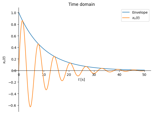
Impulse response function:

\[ x_{h}(t)=\frac{\dot x_0}{\omega_{d}}\,\mathrm{e}^{-\delta\,\omega_0\,t}\,\sin(\omega_{d}\,t). \]

The response is composed of the envelope \({\dot x_0}/{\omega_{d}}\,\exp(-\delta\, \omega_0\,t)\) and the oscillating part \(\sin(\omega_{d}\,t)\), see the figure below.

Show code cell source

Hide code cell source

import sympy as sym
t, ω_0, ω_d, d_x_0, δ= sym.symbols('t, \\omega_0, \\omega_d, d_x_0, \\delta', real=True)
data = {ω_0: 1, d_x_0: 1, δ: 0.1}

ω_d = ω_0 * sym.sqrt(1-δ**2)

envelope = d_x_0/ω_d * sym.exp(-δ*ω_0*t)

x = envelope * sym.sin(ω_d*t)

p1 = sym.plot(envelope.subs(data), (t,0,50), line_color='C0', xlabel='$t$ [s]', ylabel='$x_h(t)$', title='Time domain',
             label='Envelope', show=False)
p2 = sym.plot(x.subs(data), (t,0,50), line_color='C1', 
             label='$x_h(t)$', show=False)
p1.extend(p2)
p1.legend = True
p1.show()

Harmonic excitation

We continue with the solution of the equation of motion for the case of harmonic excitation:

\[ f(t)=F\,\mathrm{e}^{ \mathrm{i}\,\omega\,t}=F\,\underbrace{\big(\cos(\omega\,t)+ \mathrm{i}\,\sin(\omega\,t)\big)}_{\mathrm{e}^{ \mathrm{i}\,\omega\,t}}, \]

where \(F\) is the force amplitude (in general a complex value) and \(\omega\) the angular frequency of the excitation.

We determine the particular solution \(x_p(t)\) from the equation:

\[ m\,\ddot{x}_{p}(t)+c\,\dot{x}_{p}(t)+k\,x_{p}(t)=f(t), \]

by assuming a harmonic response:

\[ x_{p}(t)=X_{p}\,\,\mathrm{e}^{ \mathrm{i}\,\omega\,t}, \]

where \(X_{p}\) is the unknown complex amplitude of the particular component (sometimes also called a phasor). We continue with the derivation:

\[ -\omega^2\,m\,X_{p}\,\mathrm{e}^{ \mathrm{i}\,\omega\,t}+ \mathrm{i}\,\omega\,c\,X_{p}\,\mathrm{e}^{ \mathrm{i}\,\omega\,t}+k\,X_{p}\,\,\mathrm{e}^{ \mathrm{i}\,\omega\,t}=F\,\mathrm{e}^{ \mathrm{i}\,\omega\,t}. \]

The nontrivial solution requires \(\mathrm{e}^{ \mathrm{i}\,\omega\,t}\neq 0\), and therefore we look for the solution on the basis of the equation:

\[ -\omega^2\,m\,X_{p}+ \mathrm{i}\,\omega\,c\,X_{p}+k\,X_{p}=F, \]

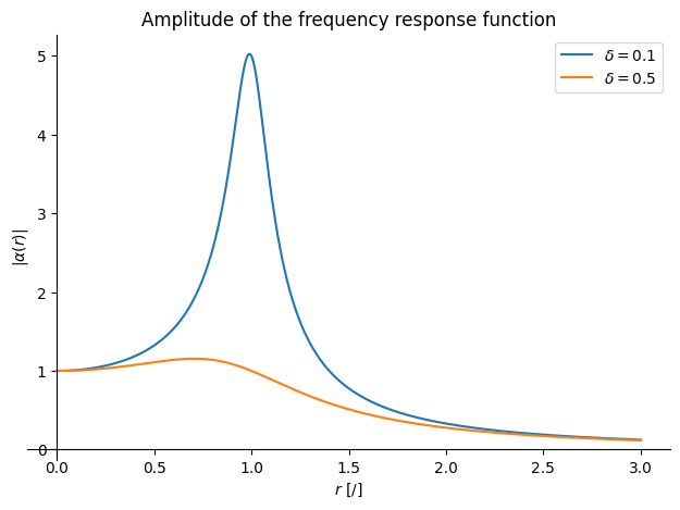
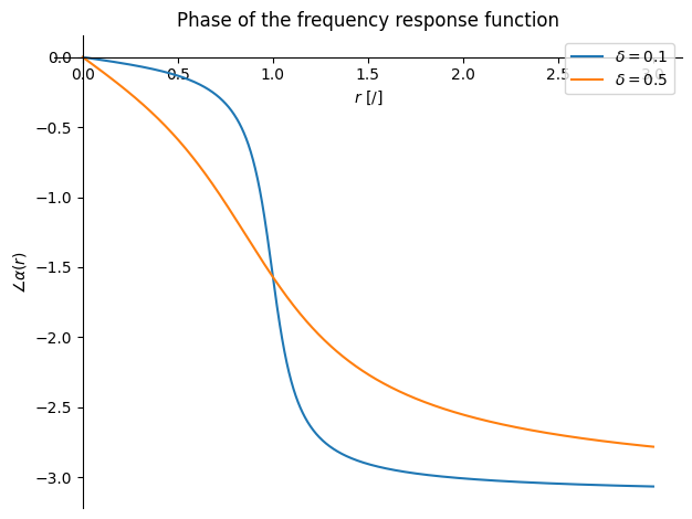
which leads to the determination of the ratio between the response \(X_p\) and the excitation \(F\), which we also call the frequency response function \(\alpha(\omega)\):

\[ \alpha(\omega)=\frac{X_{p}}{F}=\frac{1}{-\omega^2\,m+ \mathrm{i}\,\omega\,c+k}. \]

If we factor out \(1/k\), then use \(\omega_0^2=k/m\), \(c=\delta\,c_c\), \(c_c=2\sqrt{k\,m}\) and additionally introduce the frequency ratio \(r=\omega/\omega_0\), we derive:

\[ \alpha(r)=\frac{1}{k}\cdot\frac{1}{1-r^2+2\,\mathrm{i}\,\delta\,r}. \]

In what follows, we show the derived expression graphically.

Show code cell source

Hide code cell source

import sympy as sym
r, δ, k= sym.symbols('r, \\delta, k', real=True)
i = sym.I

α = 1/k/(1-r**2 + i*2*δ*r)
data = {k: 1, δ:0.1}
data2 = {k: 1, δ:0.5}

p1 = sym.plot(sym.Abs(α.subs(data)), (r,0,3), line_color='C0', xlabel='$r$ [/]', ylabel='$|\\alpha(r)|$', 
             title=f'Amplitude of the frequency response function',
             label=f'$\\delta=${δ.subs(data):2.1f}', show=False)
p2 = sym.plot(sym.Abs(α.subs(data2)), (r,0,3), line_color='C1', 
             label=f'$\\delta=${δ.subs(data2):2.1f}', show=False)
p1.extend(p2)
p1.legend = True
p1.show()

p1 = sym.plot(sym.arg(α.subs(data)), (r,0,3), line_color='C0', xlabel='$r$ [/]', ylabel='$\\angle\\alpha(r)$', 
             title=f'Phase of the frequency response function',
             label=f'$\\delta=${δ.subs(data):2.1f}', show=False)
p2 = sym.plot(sym.arg(α.subs(data2)), (r,0,3), line_color='C1', 
             label=f'$\\delta=${δ.subs(data2):2.1f}', show=False)
p1.extend(p2)
p1.legend = True
p1.show()

The particular solution is therefore:

\[ x_{p}(t)=\frac{1}{-\omega^2\,m+ \mathrm{i}\,\omega\,c+k}\,F% \,\mathrm{e}^{ \mathrm{i}\,\omega\,t}. \]

Transient response and steady-state response

First we determined the homogeneous solution \(x_{h}(t)\), which represents the transient response to some initial disturbance. The particular solution \(x_{p}(t)\) represents the solution to a stationary harmonic disturbance. The general solution is determined by the sum of both (figure below).

Frequency response function

First we will focus solely on the particular solution (but we will no longer use the subscript \(p\)):

\[ \frac{X}{F}=\frac{1}{-\omega^2\,m+ \mathrm{i}\,\omega\,c+k}. \]

Since the above expression represents the frequency response, it is called the frequency response function (FRF; see The relation between the frequency response function and the impulse response function for a description of how the FRF is obtained from the homogeneous solution).

Note

Frequency response function:

\[ \alpha(\omega)=\frac{1}{-\omega^2\,m+ \mathrm{i}\,\omega\,c+k}. \]

Using the undamped natural angular frequency \(\omega_0^2=k/m\), the damping ratio \(\delta=c/(2\,\sqrt{k\,m})\) and the frequency ratio, also called the relative frequency, \(r=\omega/\omega_0\), we obtain the frequency response in standard form:

\[ \alpha(r)=\frac{1}{k}\cdot\frac{1}{1-r^2+2\, \mathrm{i}\,\delta\,r}. \]

\(\alpha(\omega)\) is called the frequency response function, or more precisely the dimensional frequency response function. In contrast to \(\alpha(\omega)\), \(H_0(\omega)\) is defined as:

\[ \begin{split} H_0(\omega)&=\frac{X(\omega)}{X_0} \end{split} \]

and in some sources (e.g. Géradin and Rixen [2015]) it is called the nondimensional frequency response function. In the expression above, the static deflection \(X_0\) due to the static force \(F\) is defined as:

\[ X_0=\frac{F}{k}. \]

Note

The harmonic response \(X(\omega)\) can be defined with the nondimensional frequency response function as:

\[\begin{split} \begin{split} H_0(\omega)&=\frac{X(\omega)}{X_0}\\ &=\frac{k}{-\omega^2\,m+ \mathrm{i}\,\omega\,c+k}\\ &=\frac{1}{1-r^2+ \mathrm{i}\,2\,\delta\,r} \end{split} \end{split}\]

or:

\[ \alpha(\omega)=\frac{H_0(\omega)}{k}. \]

With the help of the frequency response function, the steady-state response under harmonic excitation with \(\omega_f\) can be described as:

\[ x(t)=\alpha(\omega=\omega_f)\,F\,\mathrm{e}^{ \mathrm{i}\,\omega_f\,t}. \]

Different forms of the FRF

The dimensional FRF makes sense, since the static deflection \(X_0\) is difficult to measure and, often, the excitation force and the response acceleration are measured. Instead of acceleration, we also often measure velocity and displacement. Consequently, there are different forms of the frequency response function:

Note

\[\begin{split} \begin{aligned} \alpha(\omega)&=\frac{X(\omega)}{F(\omega)},&&\textrm{receptance,}\\ Y(\omega)&=\frac{\dot{X}(\omega)}{F(\omega)}= \mathrm{i}\,\omega\,\alpha(\omega),&&\textrm{mobility,}\\ A(\omega)&=\frac{\ddot{X}(\omega)}{F(\omega)}=-\omega^2\,\alpha(\omega),&&\textrm{accelerance,}\\ \end{aligned} \end{split}\]

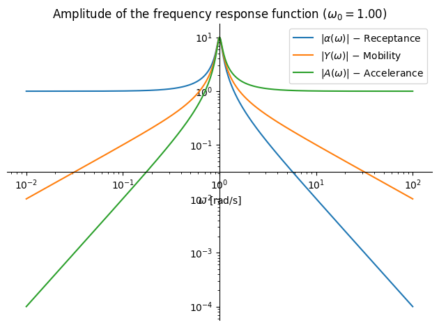
where \(\dot{X}(\omega)\) and \(\ddot{X}(\omega)\) denote the complex amplitudes of velocity and acceleration in the frequency domain. The response of the different forms of FRF is shown in the figure below:

• receptance: below resonance it converges to the static inverse of the stiffness \(1/k\), while above resonance it converges quadratically to zero,

• mobility: below resonance it converges linearly to zero, above resonance it converges linearly to zero,

• accelerance: below resonance it converges quadratically to zero, above resonance it converges to the inverse of the mass \(1/m\).

Show code cell source

Hide code cell source

import sympy as sym
ω, m, c, k= sym.symbols('\\omega, m, c, k', real=True)
i = sym.I

α = 1/(-ω**2 * m + i*ω*c + k)
data = {m: 1, c: 0.1, k: 1}

p1 = sym.plot(sym.Abs(α.subs(data)), (ω,0.01,100), line_color='C0', xlabel='$\\omega$ [rad/s]', ylabel='',  
             title=f'Amplitude of the frequency response function ($\\omega_0=${sym.sqrt(k/m).evalf(subs=data):3.2f})',
             label='$|\\alpha(\\omega)|$ $-$ Receptance', xscale='log', yscale='log', show=False)
p2 = sym.plot(sym.Abs(i*ω*α.subs(data)), (ω,0.01,100), line_color='C1', 
             label='$|Y(\\omega)|$ $-$ Mobility', xscale='log', yscale='log', show=False)
p3 = sym.plot(sym.Abs(-ω**2*α.subs(data)), (ω,0.01,100), line_color='C2', 
             label='$|A(\\omega)|$ $-$ Accelerance', xscale='log', yscale='log', show=False)
p1.extend(p2)
p1.extend(p3)
p1.legend = True
p1.show()

Note

The inverse of accelerance is the dynamic mass (\(F/\ddot{X}\)), the inverse of mobility is the mechanical impedance (\( F/\dot{X}\)) and the inverse of receptance is the dynamic stiffness (\(F/X\)).

Properties of a linear time-invariant system

The differential equation for a single-degree-of-freedom system connects the excitation (input) with the response (output):

\[ \underbrace{f(t)}_{\textrm{Excitation}}\to {\fbox{System}}\to \underbrace{x(t)}_{\textrm{Response}}. \]

A system is linear if it has the properties of additivity:

\[ f_1(t)+f_2(t) \to {\fbox{Linear system}} \to x_1(t)+x_2(t) \]

and scaling (also homogeneity):

\[ a\,f(t) \to {\fbox{Linear system}} \to a\,x(t). \]

If the system is linear, we can use the principle of superposition:

\[ a_1\,f_1(t)+a_2\,f_2(t) \to {\fbox{Linear system}} \to a_1\,x_1(t)+a_2\,x_2(t). \]

Another important property is time invariance:

\[ f(t-t_0) \to {\fbox{Time-invariant system}} \to x(t-t_0). \]

Response to periodic excitation

Writing the excitation with Fourier series

According to Fourier series in exponential (complex) form, we can write the periodic excitation \(f(t)\) as:

\[ f(t) = \sum_{n=-\infty}^{+\infty} c_n\,\mathrm{e}^{ \mathrm{i}\,n\,\omega_{p}\,t}, \]

where \(\omega_{p}\) is the fundamental angular frequency of the periodic excitation:

\[ \omega_{p} = \frac{2\pi}{T} \]

and the Fourier (complex) coefficients \(c_n\) for \(n\in \mathbb{Z}\) are defined as:

\[ c_n = \frac{1}{T}\,\int_{\tau}^{\tau+T}f(t)\,\mathrm{e}^{- \mathrm{i}\,n\,\omega_{p}\,t}\,\textrm{d} t, \]

where \(c_0\) is the average value of \(f(t)\). It also holds that \(c_{-n}=c_n^*\), where \({}^*\) denotes the complex conjugate.

Note

Since the principle of superposition holds, we can decompose the excitation into an arbitrary number of components; here we decompose the excitation into the individual terms of the Fourier series; the Fourier coefficient \(c_n\) thus defines one harmonic component.

Writing the response with the help of Fourier series

Here we continue with the computation of the solution for each harmonic component of the excitation separately (see Frequency response function):

\[\begin{split} \begin{split} X_n&=X_{0,n}\,H_0(\omega_{p}\,n)\\ &=\frac{c_n}{k}\,H_0(\omega_{p}\,n)\\ &=c_n\,\alpha(\omega_{p}\,n), \end{split} \end{split}\]

where \(c_n\) is defined above for periodic excitation by a force.

Once we have determined \(X_n\), we can compute the response of this harmonic component in time:

\[ x_n(t)=X_n\,\,\mathrm{e}^{ \mathrm{i}\,n\,\omega_{p}\,t} \]

and we return to the principle of superposition and sum the responses:

\[ x(t) = \sum_{n=-\infty}^{+\infty} x_n(t). \]

Generalization of periodic excitation to arbitrary excitation

The Fourier transform represents a generalization of Fourier series to non-periodic data as well. The derivations that we made for periodic excitation with the help of Fourier series can thus be generalized.

Note

The Fourier transform of the excitation for the transition into the frequency domain:

\[ F(\omega)=\mathcal{F}\{f(t)\} \]

decomposes the excitation into harmonic components \(F(\omega)\), which we then solve for the individual angular frequencies \(\omega\):

\[ X(\omega)=\alpha(\omega)\,F(\omega) \]

and then we make the transition back into the time domain:

\[ x(t)=\mathcal{F}^{-1}\{X(\omega)\}. \]

Excitation by a unit impulse

Let us now consider the excitation of a single-mass system by a unit impulse \(f_1(t)=\delta(t-\tau)\), where \(\delta(t)\) is the Dirac delta function (see the chapter The Dirac delta function):

\[ \Delta I_1=\lim_{\Delta \tau\to 0}\int_{\tau}^{\tau+\Delta \tau}f_1(t)\,\textrm{d}t =1. \]

The single-mass system is at rest at time \(\tau^-\), and an infinitesimal time later, \(\tau^+\), it has, because of the unit impulse \(\Delta I_1\), the velocity:

\[ \dot{x}_0 = \frac{\Delta I_1}{m}= \frac{1}{m}. \]

After the unit impulse, \(t\ge \tau\), the force \(f_1(t)\) is zero and the system responds according to the homogeneous solution with zero initial displacement \(x=0\) and \(\dot{x}=\dot{x}_0\) (see the chapter Impulse response function):

\[ h(t-\tau)=x(t)=\frac{1}{m\,\omega_{d}}\,\mathrm{e}^{-\delta\,\omega_0\,(t-\tau)}\,\sin(\omega_{d}\,(t-\tau)),\quad \textrm{for: } t>\tau, \]

where \(h(t-\tau)\) is the impulse response function.

The response to a unit impulse of a causal system depends only on past (and present) excitation, not on future excitation. All systems in this book are considered causal.

Generalization of the unit excitation to arbitrary excitation

A general excitation force (figure below) can be seen as a superposition of unit impulses multiplied by a certain constant.

Each infinitely short impulse would cause a response according to the impulse response function \(h(t-\tau)\), multiplied by the amplitude of the impulse \(f(\tau)\,\Delta\tau\). For linear systems, we sum such responses according to the principle of superposition:

\[ x(t) = \sum_{\tau}f(\tau)\,h(t-\tau)\,\Delta \tau,\quad \textrm{for: } t>\tau. \]

Because of the infinitesimally small time steps \(\Delta \tau\to0\), the sum passes into an integral:

\[ x(t) = \int_0^t\,f(\tau)\,h(t-\tau)\,\textrm{d} \tau,\quad \textrm{for: } t>\tau. \]

We call the above expression the convolution integral, the superposition integral or convolution (sometimes also the Duhamel integral).

Since the impulse response function \(h(t-\tau)=0\) for \(t<\tau\), the lower limit of the integral can be extended to \(-\infty\):

\[ x(t) = \int_{-\infty}^t\,f(\tau)\,h(t-\tau)\,\textrm{d} \tau,\quad \textrm{for: } t>\tau. \]

Furthermore, if we change the integration variable to \(\tau_1=t-\tau\) (consequently: \(\textrm{d} \tau_1=-\textrm{d} \tau\)), the limits of integration change to: \(-\infty\to+ \infty\) and \(t\to 0\):

\[ x(t) = -\int_{+\infty}^0\,f(t-\tau_1)\,h(\tau_1)\,\textrm{d} \tau_1 = \int_0^{+\infty}\,f(t-\tau_1)\,h(\tau_1)\,\textrm{d} \tau_1. \]

It follows that we can summarize a property called the commutativity of convolution:

\[ x(t) = \int_{-\infty}^{t}\,f(\tau)\,h(t-\tau)\,\textrm{d} \tau = \int_{0}^{+\infty}\,h(\tau)\,f(t-\tau)\,\textrm{d} \tau \]

or in short form:

\[ x(t) = f(t) * h(t)= h(t)*f(t), \]

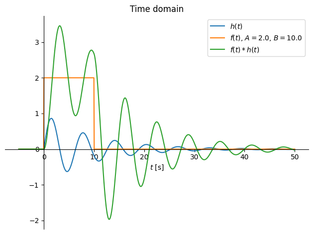
where \(*\) denotes convolution. The example below shows excitation by a step function of height \(A\) and length \(B\).

import sympy as sym
t, ω_0, ω_d, d_x_0, δ, A, B, τ = sym.symbols('t, \\omega_0, \\omega_d, d_x_0, \\delta, A, B, \\tau', real=True)
π = sym.pi
data = {ω_0: 1, d_x_0: 1, δ: 0.1, A: 2., B: 10.}

ω_d = ω_0 * sym.sqrt(1-δ**2)
envelope = d_x_0/ω_d * sym.exp(-δ*ω_0*t)
h = envelope * sym.sin(ω_d*t)*sym.Heaviside(t)

f = A*(sym.Heaviside(t)-sym.Heaviside(t-B))

fh = (f.subs(t, τ)*h.subs(t, t-τ)).subs(data)
fh = sym.integrate(fh, (τ, 0, t))

p1 = sym.plot(h.subs(data), (t,-5,50), line_color='C0', xlabel='$t$ [s]', ylabel='', title='Time domain',
             label='$h(t)$', show=False)
p2 = sym.plot(f.subs(data), (t,-5,50), line_color='C1', 
             label=f'$f(t)$, $A=${A.subs(data):3.1f}, $B=${B.subs(data):3.1f}', show=False)
p3 = sym.plot(fh, (t,-5,50), line_color='C2', 
             label='$f(t)*h(t)$', show=False)
p1.extend(p2)
p1.extend(p3)
p1.legend = True
p1.show()

And here is a slightly more detailed figure:

import numpy as np
import sympy as sym
t, ω_0, ω_d, d_x_0, δ, A, B, τ, t0 = sym.symbols('t, \\omega_0, \\omega_d, d_x_0, \\delta, A, B, \\tau, t0', real=True)
π = sym.pi
data = {ω_0: 2, d_x_0: 1, δ: 0.2, A: 0.5, B: 10., t0: 5}

ω_d = ω_0 * sym.sqrt(1-δ**2)
envelope = d_x_0/ω_d * sym.exp(-δ*ω_0*t)
h = envelope * sym.sin(ω_d*t)*sym.Heaviside(t)

f = A*(sym.Heaviside(t)-sym.Heaviside(t-B))

fh = (f.subs(t, τ)*h.subs(t, t-τ)).subs(data)
fh = sym.integrate(fh, (τ, -0, t))

x_array = np.linspace(0, data[t0], 100)
f_array = sym.lambdify(τ, f.subs(t, τ).subs(t, t0).subs(data)*h.subs(t, t-τ).subs(t, t0).subs(data))(x_array)

p1 = sym.plot(h.subs(t, t-τ).subs(t, t0).subs(data), (τ,-2,5), line_color='C0', 
              xlabel='$t$ [s]', ylabel='', title='Time domain',
             label='$h(t-\\tau)$', show=False,
             fill={'x': x_array,
                   'y1': f_array,
                   'color':'red', 'alpha':0.5})
p2 = sym.plot(f.subs(t, τ).subs(t, t0).subs(data), (τ,-2,5), line_color='C1', 
             label=f'$f(\\tau)$, $A=${A.subs(data):3.1f}, $B=${B.subs(data):3.1f}', show=False)
p5 = sym.plot_parametric((t0,fh.subs(t, t0)), (t0,4.95,5.05), line_color='r', 
             label=r'Value $\int_{-\infty}^{t='+str(data[t0])+r'\,s} f(\tau)\,h(t-\tau)\,\text{d}\tau$', show=False)
p3 = sym.plot(f.subs(t, τ).subs(t, t0).subs(data)*h.subs(t, t-τ).subs(t, t0).subs(data), (τ,-2,5), line_color='C5', 
             label=f'Integrand: $f(\\tau)\\,h(t-\\tau)$, $A=${A.subs(data):3.1f}, $B=${B.subs(data):3.1f}', show=False)
p4 = sym.plot(fh, (t,-1,8), line_color='C2', 
             label='$f(t)*h(t)$', show=False, nr_of_points=200)
p1.extend(p2)
p1.extend(p3)
p1.extend(p4)
p1.extend(p5)
p1.legend = True
p1.show()

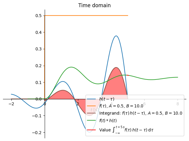
From the figure above we can see why \(h(\tau)\) is sometimes called the dynamic memory of the system; \(h(t-\tau)\) ensures that the solution at time \(t\) is influenced by what happens up to time \(t\) (see the integrand \(f(\tau)\,h(t-\tau)\) above). For the same reason, \(\tau\) is called the memory variable.

Note

If the system is non-causal and the response also depends on future excitation, the limits of integration are extended and the commutative property of convolution is:

\[ x(t) = \int_{-\infty}^{+\infty}\,f(t-\tau)\,h(\tau)\,\textrm{d} \tau = \int_{-\infty}^{+\infty}\,f(\tau)\,h(t-\tau)\,\textrm{d} \tau. \]

The relation between the frequency response function and the impulse response function

In the previous chapters, the frequency response function \(\alpha(\omega)\) and the impulse response function \(h(t)\) were presented; the first is defined in the frequency domain, the second in the time domain. In this chapter we will prove that \(h(t)\) and \(\alpha(\omega)\) form a Fourier transform pair.

The Fourier transform of the unit impulse \(f_1(t)=\delta(t)\):

\[ F_1(\omega)=\mathcal{F}\{f_1(t)\} =\int_{-\infty}^{\infty}f_1(t)\,\mathrm{e}^{- \mathrm{i}\,\omega\,t}\,\textrm{d} t =1. \]

Consequently, the unit impulse excites all frequencies equally.

The unit impulse, via the frequency response function \(\alpha(\omega)\), leads to the response \(X_1(\omega)\):

\[ X_1(\omega)=\alpha(\omega)\,\underbrace{F_1(\omega)}_{=1}=\alpha(\omega). \]

To make the transition into the time domain, we use the inverse Fourier transform:

\[\begin{split} \begin{split} x_1(t)&=\mathcal{F}^{-1}\{X_1(\omega)\}\\ &=\mathcal{F}^{-1}\{\alpha(\omega)\}. \end{split} \end{split}\]

On the other hand, the response \(x_1(t)\) to the unit impulse is also defined by the impulse response function \(x_1(t)=h(t)\), from which the following note follows.

Note

The impulse response function and the frequency response function are a Fourier pair:

\[ h(t)=\mathcal{F}^{-1}\{\alpha(\omega)\}\qquad\textrm{or}\qquad% \alpha(\omega)=\mathcal{F}\{h(t)\}. \]

Note: a Fourier pair denotes two variables, one in the time domain and the other in the frequency domain, which are connected via the Fourier transform.