2. Fourier series

2. Fourier series#

The goal of Fourier series is to describe an arbitrary (periodic) signal as a sum of harmonic signals of different fundamental periods. In this chapter we will limit ourselves to mathematically defined signals, in the following steps:

step: writing a periodic signal as a sum of harmonic signals,
step: identification of the harmonic signals from point 1,
step: generalization.

As possible additional sources, we can recommend here Shin and Hammond [2008] and Grant Sanderson: But what is a Fourier series? From heat flow to drawing with circles.

Writing a periodic signal as a sum of harmonic signals#

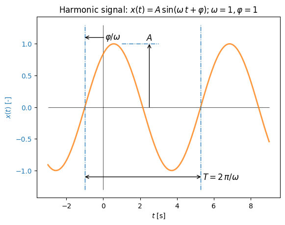
Before we get to know Fourier series in detail, let us look at the definition of a general harmonic signal:

\[ x(t) = A\,\sin(\omega\,t+\varphi), \]

where \(A\) is the amplitude, \(\omega\) the angular frequency (unit: rad/s) and \(\varphi\) the phase angle (unit: rad) with respect to the time origin. Here \(\omega=2\pi\,f\), where \(f\) is the (ordinary) frequency (unit: 1/s = Hz). A positive phase shifts the harmonic function to the left, a negative phase to the right. The period \(T\) is defined by the angular frequency: \(T=2\pi/\omega\).

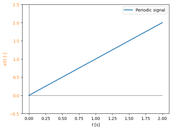
An example of a harmonic signal with amplitude \(A=1\), angular frequency \(\omega=1\) rad/s and positive phase \(\varphi=1\) rad is shown below.

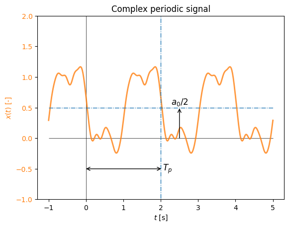
../_images/004b9cdd4b1eeec06d715503ed221cc0d2eb56ec86eba6560dc0d27fc7230790.png

Let us continue with a sum of harmonic signals, restricting ourselves to complex periodic signals (see Classification of signals), where the ratio between the frequencies of the individual harmonics is a rational number. We will additionally restrict the frequencies of the harmonic signals: if the fundamental angular frequency \(\omega_p=2\pi/T_p\) is defined by the fundamental period \(T_p\), then all the other harmonics must have an angular frequency that is a multiple of the fundamental angular frequency.

This description corresponds to a sum of harmonic signals:

\[ x(t)=\frac{a_0}{2}+\sum_{n=1}^{\infty} \left[ a_n\cos\left(\frac{2\pi\,n\,t}{T_p} \right) + b_n\sin\left(\frac{2\pi\,n\,t}{T_p} \right) \right], \]

where \(a_0\) is a constant, \(a_n\) the amplitude of the \(n\)-th cosine component and \(b_n\) the amplitude of the \(n\)-th sine component.

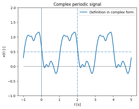
Below, let us look at an example of a harmonic signal that satisfies the restrictions of a complex periodic signal.

../_images/3b923e355fd977068fcf4d5d84229eaf554ab4be97db533de68e965cf78117c1.png

The periodic signal we looked at above is of key importance for understanding Fourier series (and later the Fourier transform, see 3. The Fourier transform). In what follows, we will first rewrite the periodic signal into complex form, since this will greatly simplify the mathematical notation and the physical clarity.

We begin the conversion into complex form with the help of Euler’s formula:

\[ \mathrm{e}^{\pm \mathrm{i}\,\alpha} = \cos\alpha \pm \mathrm{i}\,\sin\alpha, \]

where \(\mathrm{i}=\sqrt{-1}\).

If we use \(\alpha=2\pi\,n\,t/T_p\), we can write:

\[ \cos\alpha=\frac{1}{2}\mathrm{e}^{\mathrm{i}\,\alpha}+\frac{1}{2}\mathrm{e}^{-\mathrm{i}\,\alpha} \qquad\textrm{ and } \qquad \sin\alpha=-\frac{1}{2}\,\mathrm{i}\,\mathrm{e}^{\mathrm{i}\,\alpha}+\frac{1}{2}\,\mathrm{i}\,\mathrm{e}^{-\mathrm{i}\,\alpha} \]

and the function:

\[ x(t)=\frac{a_0}{2}+\sum_{n=1}^{\infty} \left[ a_n\cos\left(\frac{2\pi\,n\,t}{T_p} \right) + b_n\sin\left(\frac{2\pi\,n\,t}{T_p} \right) \right] \]

we rewrite into:

\[ x(t)=\frac{a_0}{2}+\sum_{n=1}^{\infty} \left[ a_n\left( \frac{1}{2}\mathrm{e}^{\mathrm{i}\,\alpha}+\frac{1}{2}\mathrm{e}^{-\mathrm{i}\,\alpha} \right)+ b_n\left( -\frac{1}{2}\,\mathrm{i}\,\mathrm{e}^{\mathrm{i}\,\alpha}+\frac{1}{2}\,\mathrm{i}\,\mathrm{e}^{-\mathrm{i}\,\alpha} \right) \right]. \]

Rearranging further:

\[ x(t)=\frac{a_0}{2}+\sum_{n=1}^{\infty} \left[ \left( \frac{1}{2}a_n-\frac{1}{2}\mathrm{i}\,b_n \right)\,\mathrm{e}^{\mathrm{i}\,2\pi\,n\,t/T_p} \right] +\sum_{n=1}^{\infty} \left[ \left( \frac{1}{2}a_n+\frac{1}{2}\mathrm{i}\,b_n \right)\,\mathrm{e}^{-\mathrm{i}\,2\pi\,n\,t/T_p} \right]. \]

We simplify the above expression into:

\[ x(t)=\sum_{n=-\infty}^{\infty} c_n\,\mathrm{e}^{\mathrm{i}\,2\pi\,n\,t/T_p}, \]

where:

\[\begin{split} c_n = \begin{cases} \frac{1}{2}a_n-\frac{1}{2}\textrm{i}\,b_n,& \text{if } n\geq +1,\\ \frac{1}{2}a_n, & \text{if } n = 0,\\ \frac{1}{2}a_{|n|}+\frac{1}{2}\textrm{i}\,b_{|n|},& \text{if } n\leq -1.\\ \end{cases} \end{split}\]

We find that \(c_n=c_{-n}^{*}\), where \({}^*\) denotes the complex conjugate value.

Note

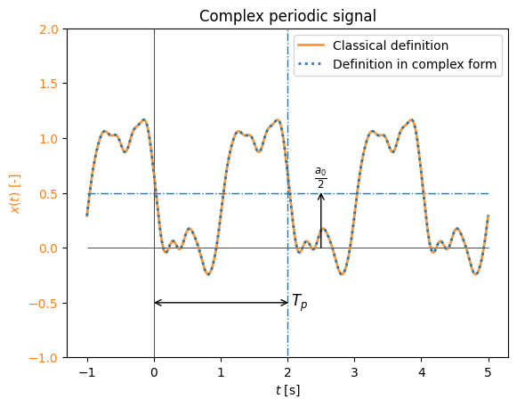
Representation of a complex periodic signal by a Fourier series with real coefficients:

\[ x(t)=\frac{a_0}{2}+\sum_{n=1}^{\infty} \left[ a_n\cos\left(\frac{2\pi\,n\,t}{T_p} \right) + b_n\sin\left(\frac{2\pi\,n\,t}{T_p} \right) \right]. \]

Note

Representation of a complex periodic signal by a Fourier series with complex coefficients:

\[ x(t)=\sum_{n=-\infty}^{\infty} c_n\,\mathrm{e}^{\mathrm{i}\,2\pi\,n\,t/T_p}. \]

Both representations above of course lead to the same result (see the example below).

Show code cell source

Hide code cell source

import numpy as np
import matplotlib.pyplot as plt


Tp = 2
t, dt = np.linspace(-0.5*Tp,2.5*Tp,301, retstep=True)
a0 = 1.
N = 10
seed = 0
rg = np.random.default_rng(seed)
a = rg.normal(size=N)*1/np.arange(1,N+1)**2 # scaled at the end so that the higher components have a smaller amplitude
b = rg.normal(size=N)*1/np.arange(1,N+1)**2

c = np.zeros(2*N+1, dtype='complex')
c[N+1:] = 0.5*a-0.5j*b
c[N] = a0/2
c[:N] = np.conj(c[N+1:])[::-1]

x1 = a0/2
for n in range(N):
    x1 += a[n]*np.cos(2*np.pi*(n+1)*t/Tp) + b[n]*np.sin(2*np.pi*(n+1)*t/Tp)

x = np.zeros(len(t), 'complex')
for n in range(-N,N+1):
    x += c[N+n]*np.exp(2j*np.pi*n*t/Tp)
x = np.real(x) # theoretically we expect only a real result (the imaginary part must be at the level of numerical error)
    
fig, ax1 = plt.subplots()
plt.title(f'Complex periodic signal')

ax1.set_xlabel('$t$ [s]')
ax1.set_ylabel('$x(t)$ [-]', color='C1')
ax1.tick_params(axis='y', labelcolor='C1')
ax1.vlines(0, -2, 2, 'k', lw=0.5)
ax1.hlines(0, np.min(t), np.max(t), 'k', lw=0.5)
ax1.plot(t, x1, label='Classical definition', c='C1', lw=2, alpha=0.8) 
ax1.plot(t, x, label='Definition in complex form', c='C0', ls=':', lw=2, alpha=1) 
ax1.vlines([Tp], -2, 2, ls='-.', lw=1)
ax1.hlines(a0/2, np.min(t), np.max(t), ls='-.', lw=1)
ax1.annotate('$\\frac{a_0}{2}$',
            xy=(2.5, 0), xycoords='data',
            ha='center', size='large',
            xytext=(2.5, a0/2+.1), textcoords='data',
            arrowprops=dict(arrowstyle='<-',
                            connectionstyle='arc3,rad=0',
                            color="k", shrinkA=0, shrinkB=0),
            )
ax1.annotate('$T_{p}$',
            xy=(0, -0.5), xycoords='data',
            va='center', size='large', 
            xytext=(Tp+0.05, -0.5), textcoords='data',
            arrowprops=dict(arrowstyle='<->',
                            connectionstyle='arc3,rad=0',
                            color="k", shrinkA=0, shrinkB=0),
            )
ax1.legend(loc=1)
plt.ylim(-1,2)
plt.show()

../_images/2be9f890bf83dbece9e50a285d36637274945f5179e102aa95edc353380cbd47.png

Identification of the harmonic signals that make up a periodic signal#

Now we can return to the original task of Fourier series: the description of an arbitrary periodic signal by a superposition of different harmonic signals.

We must answer the question of whether, in a periodic signal:

\[ x(t)=\sum_{n=-\infty}^{\infty} c_n\,\mathrm{e}^{\mathrm{i}\,2\pi\,n\,t/T_p},\qquad c_n=c_{-n}^* \]

we can identify the harmonic signal with the frequency of the \(m\)-th multiple of the fundamental frequency, i.e. \(c_m\,\mathrm{e}^{\mathrm{i}\,2\pi\,m\,t/T_p}\)?

It turns out that this is relatively simple; we begin the procedure with the integral of the periodic function \(x(t)\) multiplied by the unit harmonic function \(\mathrm{e}^{-\mathrm{i}\,2\pi\,m\,t/T_p}\), which has the negative frequency \(-m/T_p\) (instead of \(\textrm{i}\) we have \(-\textrm{i}\) in the exponent):

\[ \underbrace{\int_0^{T_p} x(t)\,\mathrm{e}^{-\mathrm{i}\,2\pi\,m\,t/T_p}\,\mathrm{d}t}_{A_m}= \underbrace{\int_0^{T_p} \sum_{n=-\infty}^{\infty} c_n\,\mathrm{e}^{\mathrm{i}\,2\pi\,n\,t/T_p} \,\,\mathrm{e}^{-\mathrm{i}\,2\pi\,m\,t/T_p}\,\mathrm{d}t}_{B_m}. \]

Since \(x(t)\) represents a known periodic signal, we can compute the integral \(A_m\). We can simplify \(B_m\) into:

\[ B_m=\int_0^{T_p} \sum_{n=-\infty}^{\infty} c_n\,\mathrm{e}^{\mathrm{i}\,2\pi\,(n-m)\,t/T_p} \,\mathrm{d}t. \]

Let us now swap the order of summation and integration and factor out the constant \(c_n\):

\[ B_m= \sum_{n=-\infty}^{\infty} c_n\,\int_0^{T_p}\mathrm{e}^{\mathrm{i}\,2\pi\,(n-m)\,t/T_p} \,\mathrm{d}t. \]

Since we are integrating a harmonic signal with a frequency that is an integer multiple of the fundamental frequency \(1/T_p\), the result is always 0, except when \(n=m\):

\[\begin{split} \int_0^{T_p}\mathrm{e}^{\mathrm{i}\,2\pi\,(n-m)\,t/T_p} \,\mathrm{d}t= \begin{cases} 0,& \text{if } n\ne m,\\ T_p,& \text{if } n= m.\\ \end{cases} \end{split}\]

It therefore follows:

\[ B_m = c_m\,T_p. \]

Since \(A_m=B_m\), it follows that the unknown Fourier coefficient \(c_m\) is defined as (it is a complex number with amplitude and phase):

\[ c_m = \frac{A_m}{T_p} = \frac{1}{T_p}\,\int_0^{T_p} x(t)\,\mathrm{e}^{-\mathrm{i}\,2\pi\,m\,t/T_p}\,\mathrm{d}t. \]

We have thus found that an individual harmonic component is relatively simple to determine; in practice the difficulty arises that the given data \(x(t)\) do not satisfy all the assumptions, in particular not the one that the harmonic is an integer multiple of the fundamental frequency. We will face these difficulties in the chapter The use of windows.

Generalization#

Fourier series are most often found defined in three forms (\(T_p\) represents the fundamental period, and \(N\) the number of harmonic components that we take into account/identify):

Fourier series in exponential (complex) form#

Note

Fourier coefficients:

\[ c_n = \frac{1}{T_p}\,\int_0^{T_p} x(t)\,\mathrm{e}^{-\mathrm{i}\,2\pi\,n\,t/T_p}\,\mathrm{d}t, \]

\[ x(t)=\sum_{n=-N}^{N} c_n\,\mathrm{e}^{\mathrm{i}\,2\pi\,n\,t/T_p},\qquad c_n=c_{-n}^*. \]

Fourier series in sine-cosine form#

Note

Fourier coefficients:

\[ a_n = \frac{2}{T_p}\,\int_0^{T_p} x(t)\,\cos(2\pi\,n\,t/T_p)\,\mathrm{d}t, \]

\[ b_n = \frac{2}{T_p}\,\int_0^{T_p} x(t)\,\sin(2\pi\,n\,t/T_p)\,\mathrm{d}t. \]

Reconstructed continuous function:

\[ x(t)=\frac{a_0}{2}+\sum_{n=1}^{N} \big(a_n\,\cos(2\pi\,n\,t/T_p)+ b_n\,\sin(2\pi\,n\,t/T_p)\big). \]

Fourier series in amplitude-phase form#

Note

Reconstructed continuous function:

\[ x(t)=\frac{A_0}{2}+\sum_{n=1}^{N} A_n\,\cos(2\pi\,n\,t/T_p-\varphi_n), \]

where the amplitude \(A_n\) and the phase \(\varphi_n\) must be determined with the help of the exponential or sine-cosine form and with the help of the transitions between the individual forms of notation:

\[\begin{split} \begin{split} c_0 &= A_0 = a_0,\\ c_n &= \frac{A_n}{2}\,\mathrm{e}^{-\mathrm{i}\,\varphi_n} = \frac{1}{2}(a_n-\mathrm{i}\,b_n),\\ c_n &= c_{-n}^*.\\ \end{split} \end{split}\]

In this book we will almost exclusively use the exponential form, since it is the most compact and the simplest to use in mathematical derivations.

Some properties of Fourier series#

Derivatives and integrals of Fourier series#

Note

The Fourier series \(x(t)\) converges to the given periodic signal \(f(t)\) if the three Dirichlet conditions are satisfied:

the signal is absolutely integrable: \(\int_0^{T_p}|f(x)|\mathrm{d}t < \infty\),
the signal has a finite number of extrema on the interval \([0,\,T_p]\),
the signal has a finite number of discontinuities on the interval \([0,\,T_p]\).

If the signal satisfies the Dirichlet conditions, the Fourier series converges to the signal at all points of the interval, including at the points of discontinuity. This is a very important result in Fourier analysis, since it allows us to represent every periodic signal as a sum of sine and cosine terms.

If the derivative \(\dot{f}(t)\) also satisfies the Dirichlet condition, then the derivative can be computed directly from the Fourier series for \(x(t)\), by differentiating the individual terms.

\[ \dot{x}(t)=\sum_{n=-N}^{N} \frac{\mathrm{i}\,2\pi\,n}{T_p}\,c_n\,\mathrm{e}^{\mathrm{i}\,2\pi\,n\,t/T_p},\qquad c_n=c_{-n}^*. \]

The analogous holds for integration:

\[ x(t)=\sum_{n=-N}^{N} \frac{T_p}{\mathrm{i}\,2\pi\,n}\,\dot{c}_n\,\mathrm{e}^{\mathrm{i}\,2\pi\,n\,t/T_p},\qquad \dot{c}_n=\dot{c}_{-n}^*, \]

where \(\dot{c}_n\) are the Fourier series constants for \(\dot{x}(t)\). For an example, see the examples that follow.

Fourier series of odd and even functions#

The function \(x(t)\) is even if:

\[ x(-t)=x(t), \]

then it also holds that:

\[ \int_{-a}^{+a} x(t)\,\mathrm{d}t=2\,\int_0^a x(t)\,\mathrm{d}t. \]

The function is odd if:

\[ x(-t)=-x(t), \]

then it also holds that

\[ \int_{-a}^{+a} x(t)\,\mathrm{d}t=0. \]

We can point out that the function \(\cos()\) is even, and the function \(\sin()\) is odd.

For the treatment that follows, the evenness/oddness of the product of functions \(x(t)\,y(t)\) is important. Whether it is even or odd depends on the evenness or oddness of the functions \(x(t)\) and \(y(t)\).

The relations are defined in the table below.

if \(x(t)\)	if \(y(t)\)	the result \(x(t)\,y(t)\) is
odd	odd	even
odd	even	odd
even	odd	odd
even	even	even

Based on the table above, we can conclude (see also Fourier series in sine-cosine form):

Note

if we are looking for the Fourier series of an even periodic function \(x(t)\), then the sine terms \(b_n\) will be equal to zero (because the product of an even and an odd function is an odd function; and the integral of an odd function is 0).
if we are looking for the Fourier series of an odd periodic function \(x(t)\), then the cosine terms \(a_n\) will be equal to zero (because the product of an odd and an even function is an odd function; and the integral of an odd function is 0).

A few examples#

Complex periodic signal#

First we will look at the complex periodic signal that we already got to know and defined above. The signal is defined by N = 10 harmonic components \(c_n\), which in the example below are known; here we will show that using the equations defined above allows us to identify them exactly.

../_images/579662ce7e5a45c3334221a7c86f848c624e5628e36634182418debc568497db.png

In the example above, the periodic signal is generated on the basis of the vector of Fourier coefficients:

array([-0.00632711+0.00521257j, -0.00434404+0.00254093j,
        0.00739907-0.00247109j,  0.01330612-0.00555366j,
        0.00502215-0.01017038j, -0.01071339-0.02491822j,
        0.00327813-0.00683724j,  0.03557904-0.12916838j,
       -0.01651311+0.00516575j,  0.06286511-0.31163723j,
        0.5       +0.j        ,  0.06286511+0.31163723j,
       -0.01651311-0.00516575j,  0.03557904+0.12916838j,
        0.00327813+0.00683724j, -0.01071339+0.02491822j,
        0.00502215+0.01017038j,  0.01330612+0.00555366j,
        0.00739907+0.00247109j, -0.00434404-0.00254093j,
       -0.00632711-0.00521257j])

We observe that the vector is complex-conjugate-symmetric about the central element. An arbitrary element can be determined solely on the basis of the time series \(x(t)\) by following the definition:

\[ c_n = \frac{1}{T_p}\,\int_0^{T_p} x(t)\,\mathrm{e}^{-\mathrm{i}\,2\pi\,n\,t/T_p}\,\mathrm{d}t, \]

which in numerical implementation (for n = 1) is:

n = 1 # Try other values too, even n > N!
sel = np.logical_and(t>=0, t<=Tp)
np.trapezoid(x[sel]*np.exp(-2j*np.pi*n*t[sel]/Tp), dx=dt)/Tp

np.complex128(0.06286511054669663+0.3116372312686761j)

In doing so, we selected (sel) only one period in the time series. Here it is worth emphasizing that we must integrate over the entire period. If the error of the numerical integration is small enough (which is the case for the example above), the result is exact to the level of the machine-precision representation in the computer.

It is worth noting that we must be very precise when implementing the derived expressions. We can quickly get a very good result; but until it is exact to the level of the machine-precision representation in the computer, there is an error somewhere in the implementation.

We would make an error if our discretization did not include the point at 0 s and the point at \(T_p\). You can test such an error by going a few lines up and making this change:

sel = np.logical_and(t>=0, t<Tp)  # wrong: t < Tp; correct is: t <= Tp

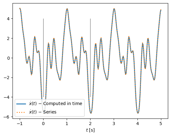
Derivative/integral of a complex periodic signal#

Let us continue with the example and look at the time derivative. In the code below we show that the Fourier series of the time derivative is indeed equal to the Fourier series in which we have simply differentiated each of the terms of the Fourier series of the original data.

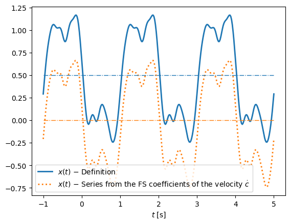
../_images/3c2d0f42cb14ed96961f6f8ce9ee0948ce2136a34ae29f88a206f8f4eb27e8db.png

We can continue the example above and identify the original displacement \(x(t)\) from the Fourier series for the velocity \(\dot x(t)\) (see the code and figure below). When integrating, we have a problem in the case of the Fourier coefficient with frequency 0 (the static component); in the code below we simply skip this frequency, since we cannot determine it. We would have a similar problem in time; if we integrate the indefinite integral, then when integrating we need an initial value. In the figure below, a deviation of the size of the static component therefore appears between the two approaches.

../_images/b1f5738b5ea404f76fc18f033d273401249ab5717c9eefbdc71fe6217cb59dd0.png

Periodic signal#

Here we will look at a periodic signal that, however, is not complex periodic with a finite number of harmonic components. An example of such a function is a rising sawtooth, shown in the figure below.

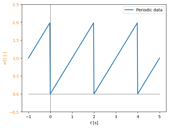
../_images/de914546bfbf5302a06bb9916f249ce82e15e2af18bb7b3ef0c64996c39a13a9.png

Even though the signal is not complex periodic, while the theory of Fourier series was derived under this assumption, let us try to identify the harmonic components. We first do this on a discrete time series. Let us focus on the part of the data that repeats:

../_images/48d765b9585fedd8229a075da852ece55d0c358df6256efafa4c24660c47595c.png

Let us identify the Fourier coefficients:

N = 10
c = np.zeros(2*N+1, dtype='complex')
n = np.arange(-N,N+1)
for i in n:
    c[i+N] = np.trapezoid(x*np.exp(-2j*np.pi*i*t/Tp), dx=dt)/Tp
c

array([-3.90312782e-16-0.03077684j, -3.83373888e-16-0.03442023j,
       -4.96130914e-16-0.03894743j, -2.65412692e-16-0.04473743j,
        1.52655666e-16-0.05242184j, -5.37764278e-17-0.06313752j,
       -4.51028104e-17-0.07915815j, -6.67868538e-17-0.10578895j,
       -6.24500451e-17-0.15894545j, -1.38777878e-17-0.31820516j,
        1.00000000e+00+0.j        , -1.38777878e-17+0.31820516j,
       -6.24500451e-17+0.15894545j, -6.67868538e-17+0.10578895j,
       -4.51028104e-17+0.07915815j, -5.37764278e-17+0.06313752j,
        1.52655666e-16+0.05242184j, -2.65412692e-16+0.04473743j,
       -4.96130914e-16+0.03894743j, -3.83373888e-16+0.03442023j,
       -3.90312782e-16+0.03077684j])

On the basis of the identified Fourier coefficients, we do not obtain a result equal to the given data (the rising sawtooth), but rather a new signal that is complex periodic:

\[ x(t)=\sum_{n=-N}^{N} c_n\,\mathrm{e}^{\mathrm{i}\,2\pi\,n\,t/T_p},\qquad c_n=c_{-n}^*. \]

The concrete numerical code is shown below (here we used a new numerical array x_r, to distinguish it from the data in the form x):

x_r = np.zeros(len(t), 'complex')
for n in range(-N,N+1):
    x_r += c[N+n]*np.exp(2j*np.pi*n*t/Tp)
x_r = np.real(x_r) # theoretically we expect only a real result (the imaginary part must be at the level of numerical error)

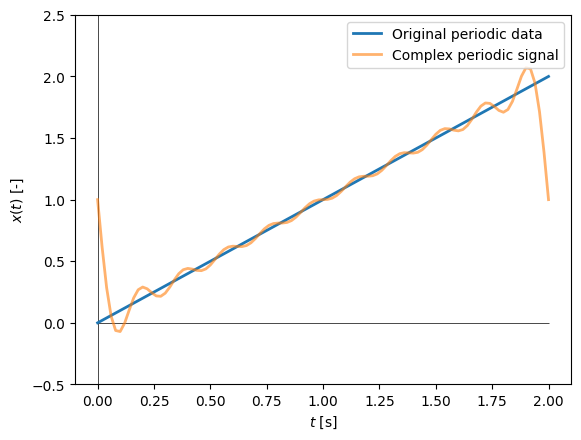
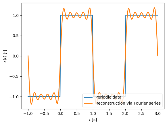
../_images/f66205f14b5ac4fe1c1bcb1723a7d061ee3f0aef98c5b398d1ccd122e2eb0748.png

We observe that the identified complex periodic signal describes the original periodic signal relatively well. If we increased the number of harmonic (\(N\)) components, the identified function would fit the original data better, but at the point of discontinuity we would still have a deviation. The deviation at the point of discontinuity is known under the term Gibbs phenomenon. In truth, most engineering applications are continuous, and therefore the Gibbs phenomenon usually has no major significance in practice.

Analytical treatment of periodic signals#

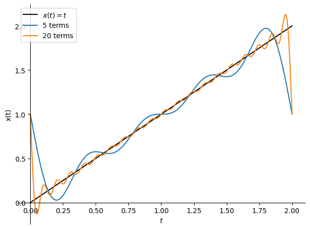
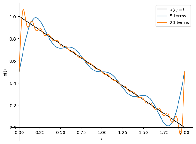
Above, we computed the Fourier series on discrete data, so we are limited in how many harmonic components we can compute (N < len(t)/2; why \(N\) is tied to the length of the time series we will learn later). Here we will look at the treatment of continuous systems and determine the Fourier series with the help of symbolic derivation. As an example of a periodic signal we will choose a rising sawtooth, which will be proportional to time t, with period Tp:

import sympy as sym
sym.init_printing()

t, T_p = sym.symbols('t, T_p', real=True)
x_r = sym.fourier_series(t, limits=(t, 0, T_p))

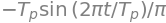
The series composed of the first 5 terms is therefore:

x_r.truncate(5)

../_images/07b8b82e492fd87a3117678cf5e6057bf54e92ad6793ec0c703662eec4ace1c2.png

We can also compute an individual term ourselves:

n = 1
c_n = sym.integrate(t*sym.exp(-sym.I*2*n*sym.pi*t/T_p), (t, 0, T_p)).simplify()/T_p
c_n

../_images/036c97e83a7f4b03ef5f8ddd43e58bb00e2c3b8a89a538289487918dea404d3c.png

To obtain the harmonic component, we must multiply c_n by the corresponding positive and negative frequency:

sym.simplify(c_n*sym.exp(sym.I*2*sym.pi*n*t/T_p)+sym.conjugate(c_n)*sym.exp(-sym.I*2*sym.pi*n*t/T_p))

../_images/8396e0281c8833ba4f384f170b28961f48de0f7ff474d55da08f2da04d43c7f7.png

The figure for T_p = 2 and a different number of terms in the series:

../_images/99dc2f8a7b1c9d7c070ca85601edc5d4ed9fc21713088caa651d6ffef28e5f71.png

The Dirac delta function#

The Dirac delta function is shown in the figure below: over the entire domain, except at the value \(t=0\), where it goes to infinity, it has the value zero; the integral of the Dirac delta function is equal to 1.

dirac-delta

Note

The Dirac delta function is defined by:

\[ \delta(t)=0 \quad\textrm{ for } t\ne 0 \qquad\textrm{ and } \qquad \int_{-\infty}^{+\infty}\delta(t)\,\textrm{d}t=1. \]

Note: this is actually not an ordinary function, but a so-called generalized function.

Since the integral of the Dirac delta function is 1, it is sometimes also called the unit-impulse function, also defined as:

\[\begin{split} \delta_{\varepsilon}= \begin{cases} \frac{1}{\varepsilon}&\textrm{ for }\quad -\frac{\varepsilon}{2}\le t\le+\frac{\varepsilon}{2},\\ 0& \textrm{otherwise}. \end{cases} \end{split}\]

When defining the unit impulse, we can also help ourselves with two unit-step functions. The unit-step function (also the Heaviside function) is defined as:

\[\begin{split} u(t)= \begin{cases} 1&\textrm{ for }\quad t>0,\\ 0& \textrm{otherwise}. \end{cases} \end{split}\]

We thus define the unit impulse with the help of two unit-step functions:

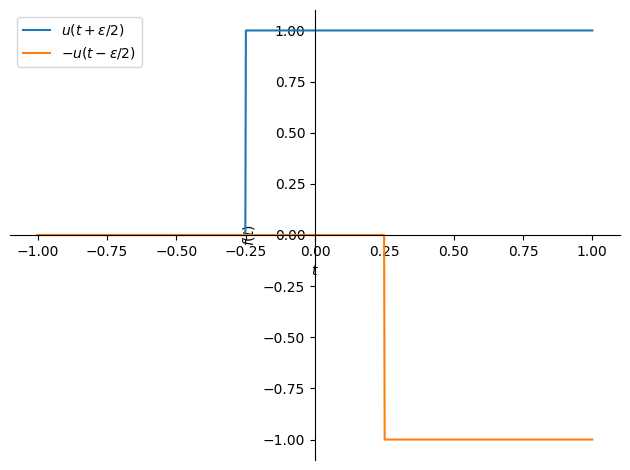
../_images/84ddea1752827fb361dbdd6ee9c77ab856babbfa42588cfcb6a494038efda469.png

We arrive at the unit impulse by weighted summation:

\[ \delta_{\varepsilon}=\frac{1}{\varepsilon}\Big(u\big(t+\frac{\varepsilon}{2}\big)-u\big(t-\frac{\varepsilon}{2}\big)\Big). \]

Let us look at how we convert the step function into a unit impulse:

import sympy as sym
t, ε = sym.symbols(r't, \varepsilon')
data = {ε: 0.5}
unit_step = sym.Heaviside(t+ε/2) # Here we must normalize correctly (H0), see help!
δ_ε = 1/ε * (unit_step-unit_step.subs(ε, -ε))
δ_ε

../_images/1213f42d69f14f375d5a1aa1b0a3e79e4f78a89aae750fb5acff6062437a37f9.png

../_images/06297c247317cd9ef5aa1ada3ce4c2549284fcd41219eba2c671c1a8b3013c27.png

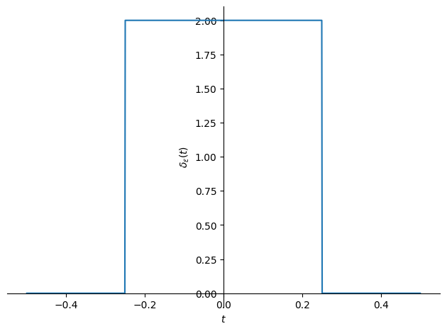
and then we integrate (the result is, as expected, equal to 1; change \(\varepsilon\) in data above!):

sym.integrate(δ_ε.subs(data), (t, -sym.oo, sym.oo))

../_images/a0aade88abe59df89dfd84058176870604a51ffdd41ddc5f8928f7afd5fdad86.png

Between the Dirac delta function and the unit step, the following relation also holds (\(u(t)\) is the step function):

\[ \delta(t)=\lim_{\varepsilon\rightarrow 0}\delta_{\varepsilon}(t)=\frac{\textrm{d}}{\textrm{d}t}u(t). \]

Properties of the Dirac delta function#

Note

It is even: \(\delta(t)=\delta(-t)\).
Sifting property \(-\) this means that the integral of an ordinary function \(x(t)\) and the shifted Dirac function \(\delta(t-a)\) gives the value of the function \(x(a)\):\(\int_{-\infty}^{+\infty}x(t)\,\delta(t-a)\,\textrm{d}t= x(a)\).
\(\int_{-\infty}^{+\infty}\mathrm{e}^{\pm\textrm{i}\,2\pi\,a\,t}\,\textrm{d}t= \delta(a)\) or also: \(\int_{-\infty}^{+\infty}\mathrm{e}^{\pm\textrm{i}\,a\,t}\,\textrm{d}t= 2\pi\,\delta(a)\), for the proof see Bendat and Piersol [2011], Shin and Hammond [2008] (p. 40).
\(\delta(a\,t)=\delta(t)/|a|\).
\(\int_{-\infty}^{+\infty}f(t)\,\delta^{(n)}(t-a)\,\textrm{d}t= (-1)^n\,f^{(n)}(a)\), where \(n\) denotes the derivative.

The falling sawtooth and its derivative#

Let us assume a periodic signal in the form of a falling sawtooth, as shown below:

../_images/10fc1d42d19dac46a5caa31c3d29df3c99d2ba4ca77a054519f59fe5438710a6.png

The Fourier series of the falling sawtooth signal is defined as:

\[ x(t) = \frac{1}{2}+\frac{1}{\pi}\sum_{n=1}^{\infty}\frac{1}{n}\sin\left(\frac{2\pi\,n\,t}{T_p}\right). \]

Or with the help of symbolic derivation:

import sympy as sym
sym.init_printing()

t, T_p = sym.symbols('t, T_p')
data = {T_p: 2}
x = 1-t/T_p
x_r = sym.fourier_series(x, limits=(t, 0, T_p))

x_r.truncate(5)

../_images/d4074c41581ce99b1615f61dac41fa180156538128a4795f63676401d4d6475e.png

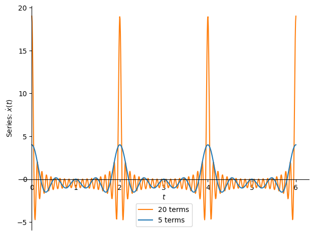
If we differentiate the falling sawtooth function in time, the result is equal to:

\[ \dot x(t) = -\frac{1}{T_p} + \sum_{n=-\infty}^{+\infty}\delta(t-n\,T_p); \]

but since we can also differentiate the series, it also holds that:

\[ \dot x(t) = \frac{2}{T_p}\sum_{n=1}^{\infty}\cos\left(\frac{2\pi\,n\,t}{T_p}\right). \]

With the help of the last two equations, we can derive the expression for the train of impulses:

Note

a periodic train of impulses has constant coefficients (\(2/T_p\)) in the form of a Fourier series:

\[ \sum_{n=-\infty}^{+\infty}\delta(t-n\,T_p) = \frac{1}{T_p} +\frac{2}{T_p}\sum_{n=1}^{\infty}\cos\left(\frac{2\pi\,n\,t}{T_p}\right). \]

We will need this finding when we deal with the sampling of signals.

../_images/3720e7053869f2890ea34ba831de312d507fc902bd57126d5e6219b1f9e011f2.png

Amplitude and phase spectrum#

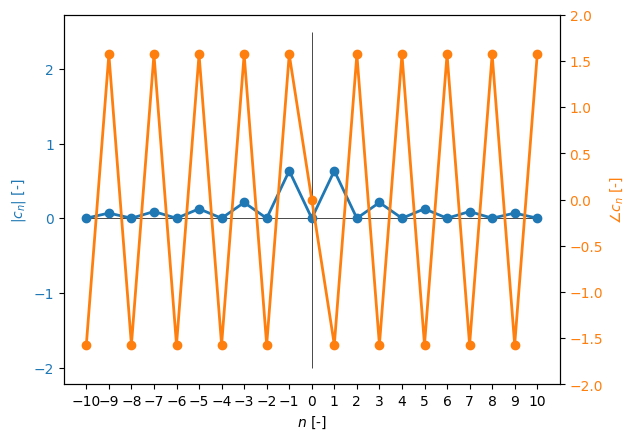
The Fourier coefficients \(c_n\) that we consider in Fourier series represent the amplitude and phase information about a particular harmonic component. Let us look at the example of a periodic square wave in the figure below:

../_images/30b3e4beec158b45a185bff4448f44d4e30685b0003b3835ff7f0e1fe53fed41.png

When preparing the data above, we computed the Fourier coefficients \(c\):

array([-3.29597460e-17-1.98252732e-03j, -3.12250226e-17+6.99121564e-02j,
       -1.70002901e-16-1.58622479e-03j,  3.08780779e-16+9.03023227e-02j,
        1.17961196e-16-1.18979483e-03j,  4.85722573e-17+1.26862832e-01j,
       -4.16333634e-17-7.93259458e-04j,  6.59194921e-17+2.11929286e-01j,
       -6.93889390e-18-3.96649155e-04j,  6.59194921e-17+6.36527232e-01j,
        0.00000000e+00+0.00000000e+00j,  6.59194921e-17-6.36527232e-01j,
       -6.93889390e-18+3.96649155e-04j,  6.59194921e-17-2.11929286e-01j,
       -4.16333634e-17+7.93259458e-04j,  4.85722573e-17-1.26862832e-01j,
        1.17961196e-16+1.18979483e-03j,  3.08780779e-16-9.03023227e-02j,
       -1.70002901e-16+1.58622479e-03j, -3.12250226e-17-6.99121564e-02j,
       -3.29597460e-17+1.98252732e-03j])

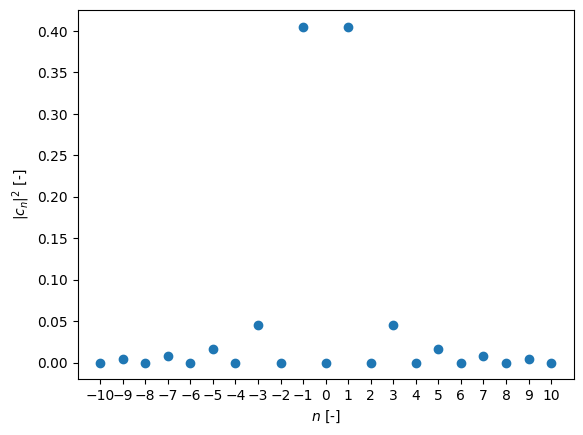
The Fourier coefficients can be shown in graphical form. If we show the amplitude of the complex number \(|c|\), then we speak of the amplitude spectrum: for a particular multiple of the fundamental frequency \(1/T_p\) we show the amplitude content of the harmonic component. Similarly, we speak of the phase spectrum if we show \(\angle c_n\).

../_images/baeca1c080d92e8cefe3c51d10a679724978afe6ad4170075cb35ee5bcd276cb.png

Parseval’s theorem and the power spectrum#

Parseval’s theorem#

If \(x(t)\) is the voltage measured across a resistor of resistance \(1\,\Omega\), then the instantaneous power is equal to \(P(t)=R\,x^2(t)\), and the average power of a periodic signal within one period is:

\[ \frac{1}{T_p}\int_0^{T_p}x^2(t)\,\textrm{d}t; \]

since \(x(t)=\sum_{n=-\infty}^{\infty}c_n\,\mathrm{e}^{\mathrm{i}\,2\pi\,n\,t/T_p}\) and \(x^2(t)=x(t)\,x^*(t)\), the average power is also defined as:

\[ \frac{1}{T_p}\int_0^{T_p}x^2(t)\,\textrm{d}t= \frac{1}{T_p}\int_0^{T_p}\sum_{n=-\infty}^{\infty}c_n\,\mathrm{e}^{\mathrm{i}\,2\pi\,n\,t/T_p}\,\sum_{m=-\infty}^{\infty}c_m^*\,\mathrm{e}^{-\mathrm{i}\,2\pi\,m\,t/T_p}\,\textrm{d}t, \]

which we simplify into:

\[ \frac{1}{T_p}\int_0^{T_p}x^2(t)\,\textrm{d}t= \frac{1}{T_p}\sum_{n=-\infty}^{\infty}\,\sum_{m=-\infty}^{\infty}c_n\,c_m^*\,\int_0^{T_p}\mathrm{e}^{\mathrm{i}\,2\pi\,(n-m)\,t/T_p}\,\textrm{d}t. \]

The integral of a harmonic signal over a complete period is always zero, except when the frequency is 0. When the frequency is equal to 0, the integrand is equal to 1 and the integral \(T_p\):

\[\begin{split} \int_0^{T_p}\mathrm{e}^{\mathrm{i}\,2\pi\,(n-m)\,t/T_p}\,\textrm{d}t= \begin{cases} T_p,&\textrm{if}\quad m=n,\\ 0&\textrm{otherwise.}\\ \end{cases} \end{split}\]

Note

The Parseval theorem, or also Parseval’s identity, follows:

\[ \frac{1}{T_p}\int_0^{T_p}x^2(t)\,\textrm{d}t= \sum_{n=-\infty}^{\infty}c_n\,c_n^*, \]

which connects the average power in time with the power in the frequency domain.

Let us look at a concrete example:

T_p = 2
t, dt = np.linspace(0,T_p,101, retstep=True)
a0 = 1.
N = 10
seed = 0
rg = np.random.default_rng(seed)
a = rg.normal(size=N)*1/np.arange(1,N+1)**2 # scaled at the end so that the higher components have a smaller amplitude
b = rg.normal(size=N)*1/np.arange(1,N+1)**2

c = np.zeros(2*N+1, dtype='complex')
c[N+1:] = 0.5*a-0.5j*b
c[N] = a0/2
c[:N] = np.conj(c[N+1:])[::-1]

x = np.zeros(len(t), 'complex')
for n in range(-N,N+1):
    x += c[N+n]*np.exp(2j*np.pi*n*t/T_p)
x = np.real(x) # theoretically we expect only a real result (the imaginary part must be at the level of numerical error)

The value from time:

np.trapezoid(x**2,dx=dt)/T_p

../_images/c49a006ed2f4ae150e6dd785428ffb8c08313d5ae088548b4a295aebac198e9c.png

The value based on the Fourier coefficients:

np.dot(c,np.conjugate(c))

np.complex128(0.4912052334566629+0j)

As expected, we get the same value (to the level of numerical error)!

Power spectrum#

Parseval’s theorem defines the average power as the sum of the squares of the Fourier coefficients, i.e. the frequency components. The display of the squares of the individual frequency components is called the power spectrum. Here it must be emphasized that the power spectrum loses the phase information and is always defined by real values.

../_images/245f2391f1f1256b01ba3bd7292b88b900e6549536bff1cc636d5772adabee98.png

2. Fourier series

Contents

2. Fourier series#

Writing a periodic signal as a sum of harmonic signals#

Identification of the harmonic signals that make up a periodic signal#

Generalization#

Fourier series in exponential (complex) form#

Fourier series in sine-cosine form#

Fourier series in amplitude-phase form#

Some properties of Fourier series#

Derivatives and integrals of Fourier series#

Fourier series of odd and even functions#

A few examples#

Complex periodic signal#

Derivative/integral of a complex periodic signal#

Periodic signal#

Analytical treatment of periodic signals#

The Dirac delta function#

Properties of the Dirac delta function#

The falling sawtooth and its derivative#

Amplitude and phase spectrum#

Parseval’s theorem and the power spectrum#

Parseval’s theorem#

Power spectrum#