3. The Fourier transform#
While Fourier series are limited to periodic data, the goal of the Fourier transform is generalization to non-periodic data. The idea is to achieve this by extending the period \(T_p\) to infinity. In what follows, we will look at the details.
The computation of the Fourier series (2. Fourier series) is based on the period \(T_p\); the integral for computing the coefficients can be defined from \(-T_p/2\) to \(+T_p/2\):
where \(\omega_p=2\pi/T_p\) is the fundamental angular frequency. When \(T_p\) becomes large and goes to infinity \(T_p\rightarrow \infty\), the fundamental angular frequency goes to zero: \(\omega_p\rightarrow 0\). To avoid problems with division by \(\infty\), we multiply the above expression by \(T_p\), use \(\omega_n=n\,\omega_p\) and continue:
Assuming that the limit exists, we write the Fourier transform (also the Fourier integral):
where instead of \(\omega_{n}\) we wrote \(\omega\), since the frequency is now continuously defined. \(X(\omega)\) represents the amplitude frequency density, since \(c_n\,T_p=c_n/\Delta f\), where \(\Delta f\) is the frequency bandwidth. We denote the Fourier transform by \(\mathcal{F}\{\}\).
Let us now also look at the reconstructed continuous function, when \(T_p\rightarrow \infty\):
The given expression is continuous and we call it the inverse Fourier transform. We denote it by \(\mathcal{F}^{-1}\{\}\):
In the expression above we used \(\textrm{d}f=\textrm{d}\omega/(2\pi)\).
Note
Here we repeat once more the Fourier transform and its inverse, written in angular frequency:
Note
In numerical methods, however, the frequency is more often defined in ordinary frequency; then the Fourier transform and its inverse are defined as:
A few examples of the Fourier transform#
The Dirac delta function#
First let us look at the Fourier transform of the Dirac delta function \(\delta(t)\):
On the basis of the derivation above, we conclude that the Dirac delta function is infinitely short in time and infinitely wide in the frequency domain (it occupies the entire spectrum, i.e. all frequencies). The reverse would also hold: if we defined the delta function in the frequency domain, it would be infinitely narrow, and infinitely wide in time. We will return to this concept later.
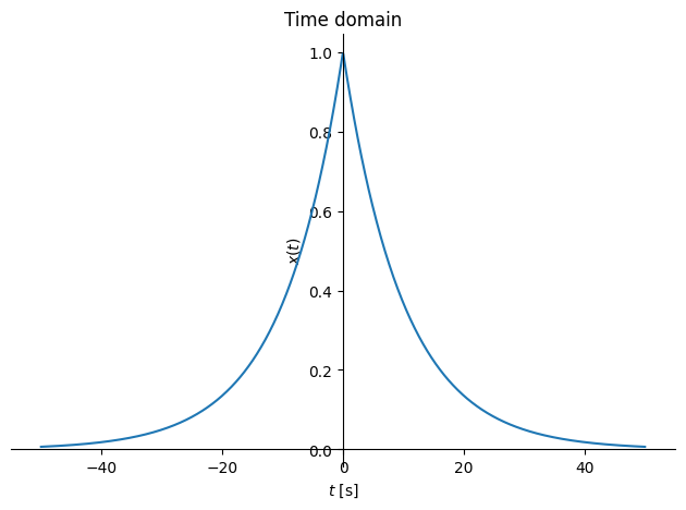
Symmetric exponentially decaying function#
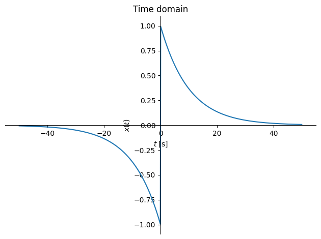
Let us now look at the symmetric exponentially decaying function \(x(t)\):
Fourier transform:
We observe that at the frequency 0 Hz the amplitude is \(X(0)=2/\eta\), and at the frequency \(f_{1/2}=|\eta/(2\pi)|\) it falls to half of the initial amplitude. The parameter \(\eta\) defines the time spread; the larger the value of \(\eta\), the faster the function will converge to zero in the time domain and the slower in the frequency domain. Similarly to the delta function, we therefore find that a small time spread results in a large frequency spread and vice versa.
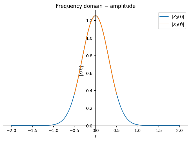
Let us now look at an example in time and frequency:
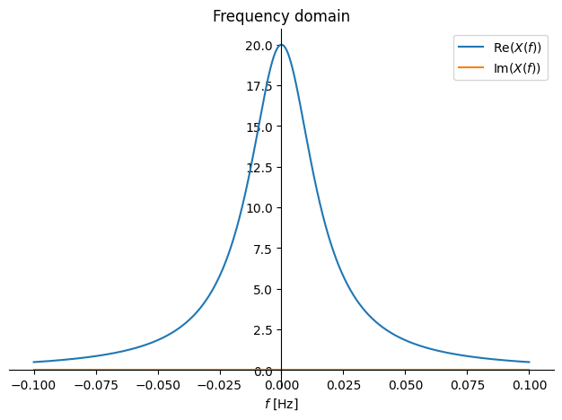
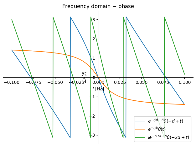
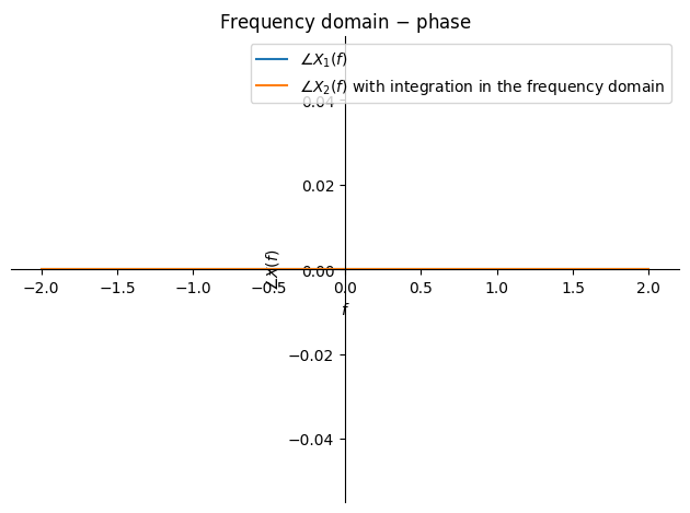
In the example above we observe that the symmetric exponential function results in a Fourier transform that has only a non-zero real component. This holds in general for all even functions; for odd functions the reverse would hold: the imaginary component would be non-zero (figure below). We already found something similar with the Fourier series of even and odd functions (for more, see Fourier series of odd and even functions).
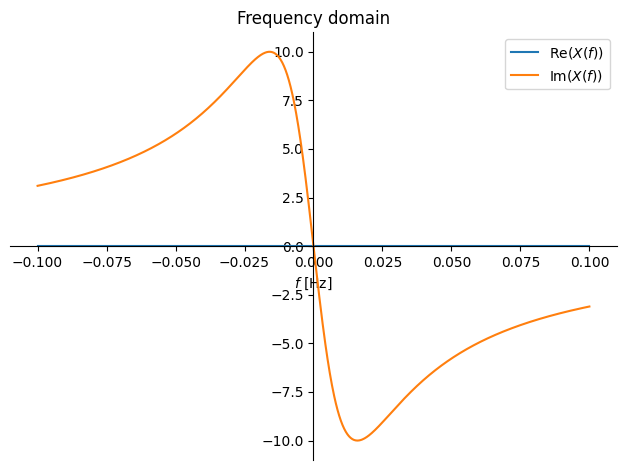
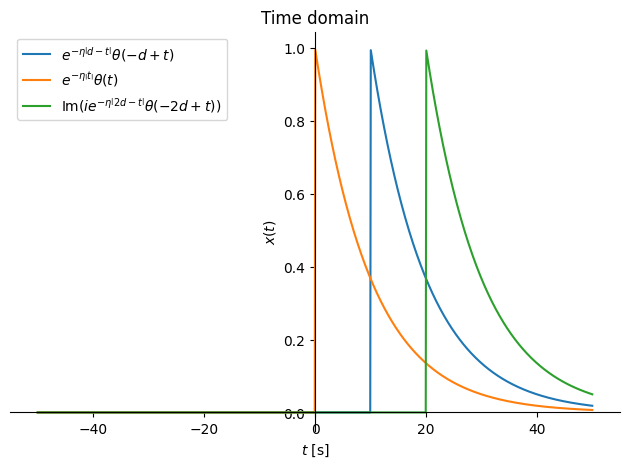
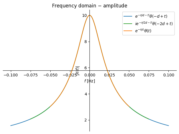
It is worth emphasizing, however, that in general real signals \(x(t)\) become complex after the Fourier transform; their amplitude is an even function and their phase an odd function (figure below; \(\theta(t)\) denotes the unit-step function). Time signals can in general be of complex form, and then in the frequency domain we generally do not observe the evenness/oddness of the amplitude or phase (try changing the code below).
Sine function#
Let us assume a sine function:
which we rewrite into:
and then continue with the computation of the Fourier transform:
import sympy as sym
A, t, f = sym.symbols('A, t, f', real=True)
p = sym.symbols('p', real=True, positive=True)
i = sym.I
π = sym.pi

x = A*(sym.exp(i*2*π*p*t)-sym.exp(-i*2*π*p*t))/(2*i)
X = sym.fourier_transform(x, t, f)
X
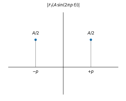
In the above symbolic derivation, \(\mathcal{F}_{t}[\cdot]\) represents the Fourier transform. Given the properties of the Dirac delta function (see Properties of the Dirac delta function), we know that \(\mathcal{F}_{t}\left[\mathrm{e}^{-2\,\textrm{i}\,\pi\,p\,t}\right]\left(f\right)=\delta(p+f)\), from which it follows:
which is shown in the figure below.
Rectangular impulse#
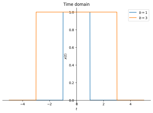
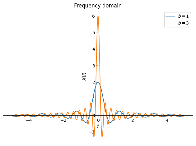
Let us assume a rectangular function:
which in the case of the Fourier transform leads to the expression:
which we can rewrite into:
The above expression clearly shows: as \(f\) tends to 0, \(X(f)\) tends to \(2\,a\,b\); otherwise it oscillates in the frequency domain with frequency \(1/b\). We can see some characteristics from the figure below: again we observe that the wider the data are in time, the narrower they are in frequency.
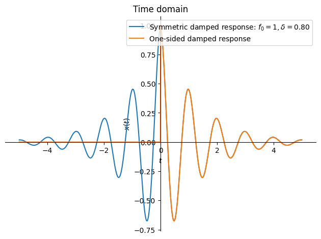
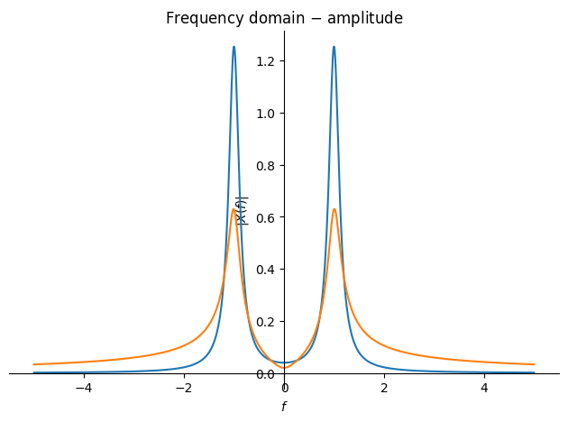
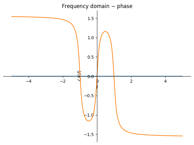
Damped response#
Here we will first look at the symmetric damped response:
and then the one-sided damped response:
We derive the Fourier transform for both damped responses (and then show it):
import sympy as sym
t, f = sym.symbols('t, f', real=True)
δ = sym.symbols('\\delta', real=True, positive=True)
f_0 = sym.symbols('f_0', real=True, positive=True)
i = sym.I
π = sym.pi

data = {δ: 0.1, f_0: 1}
x_1 = sym.exp(-δ*sym.Abs(t))*sym.cos(2*π*f_0*t)
x_2 = sym.Heaviside(t)*sym.exp(-δ*t)*sym.cos(2*π*f_0*t)
X_1 = sym.fourier_transform(x_1, t, f)
X_2 = sym.fourier_transform(x_2, t, f)
X_2
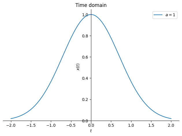
Gaussian impulse#
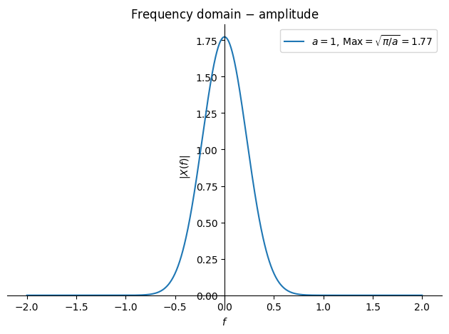
The Gaussian window has a very important place in various theoretical derivations (e.g. probability distribution, windows, wavelet transform), and therefore we will look here at its form in the frequency domain. Let us first define:
We derive the Fourier transform (below), which results in:
import sympy as sym
t, f = sym.symbols('t, f', real=True)
a = sym.symbols('a', real=True, positive=True)

x = sym.exp(-a*t**2)
X = sym.fourier_transform(x, t, f)
X
We then also show the result graphically (since the Gaussian function is even, the phase in the frequency domain is equal to 0):
Properties of the Fourier transform#
Linearity#
Note
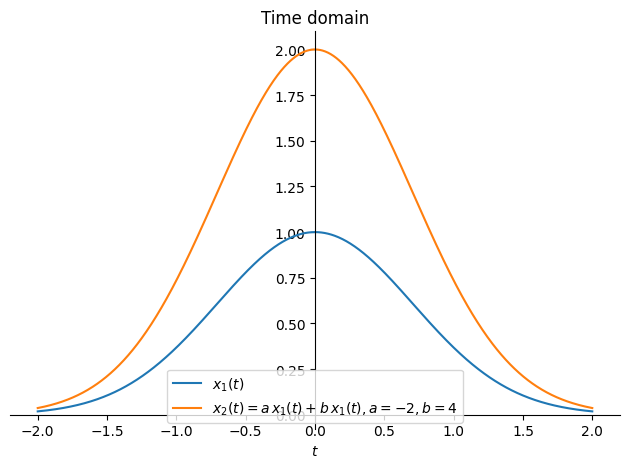
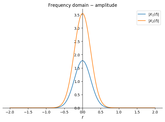
The Fourier transform is linear, which means:
And the derivation:
import sympy as sym
t, f = sym.symbols('t, f', real=True)
a, b = sym.symbols('a, b', real=True, positive=True)
x = sym.Function('x')
y = sym.Function('y')
i = sym.I
π = sym.pi

A = sym.integrate(( a*x(t) + b*y(t) )*sym.exp(-i*2*π*f*t), (t, -sym.oo, +sym.oo))
A
We expand the expression; since \(a\) and \(b\) are constants, we confirm linearity:
sym.expand(A)
Below, let us look at a concrete example.
Time scaling#
Note
Time scaling is defined as \(a\,t\) and has the following effect on the Fourier transform:
And the derivation (for positive \(a\)):
import sympy as sym
t, f, τ = sym.symbols('t, f, tau', real=True)
a = sym.symbols('a', real=True, positive=True)
x = sym.Function('x')
i = sym.I
π = sym.pi
X = sym.integrate(x(a*t)*sym.exp(-i*2*π*f*t), (t, -sym.oo, +sym.oo))

sym.Eq(X, X.transform(a*t, τ))
Time scaling becomes important, for example, when we observe the same event with two different clocks.
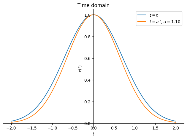
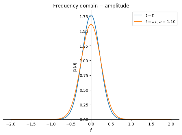
The Fourier transform of a time-scaled function is equal to the appropriately corrected unscaled Fourier transform:
X_2
(X_1/a).subs(f, f/a).subs(data)
Time reversal#
Note
Time reversal has the following effect on the Fourier transform:
And the derivation:
import sympy as sym
t, f, τ = sym.symbols('t, f, tau', real=True)
a = sym.symbols('a', real=True, positive=True)
x = sym.Function('x')
i = sym.I
π = sym.pi
X = sym.integrate(x(-t)*sym.exp(-i*2*π*f*t), (t, -sym.oo, +sym.oo))

sym.Eq(X, X.transform(-t, τ))
Time shifting#
Note
The time shift is defined by \(t_0\) and has the following effect on the Fourier transform:
And the derivation:
import sympy as sym
t, t_0, f, τ = sym.symbols('t, t_0, f, tau', real=True)
a = sym.symbols('a', real=True, positive=True)
x = sym.Function('x')
i = sym.I
π = sym.pi
X = sym.integrate(x(t-t_0)*sym.exp(-i*2*π*f*t), (t, -sym.oo, +sym.oo))

sym.Eq(X, X.transform(t-t_0, τ))
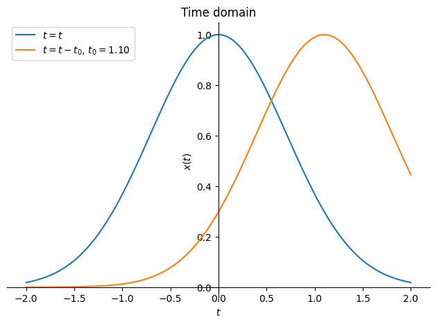
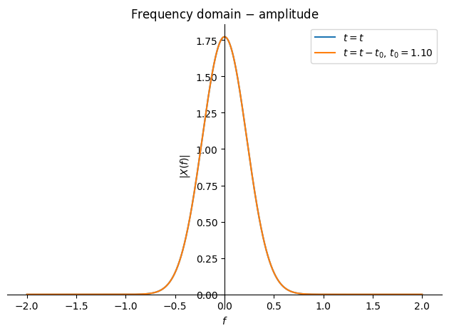
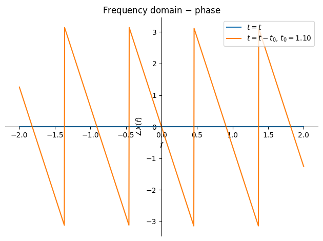
We observe that the term \(\mathrm{e}^{-\textrm{i}\,2\pi\,f\,t_0}\) can be factored out of the integral.
Time shifting becomes important when we deal with delayed measurements (e.g. if we measure one signal with a delay relative to the others): see the example below.
Amplitude modulation (also frequency shifting)#
Note
Amplitude modulation is defined by \(\mathrm{e}^{\textrm{i}\,2\pi\,f_0\,t}\) and has the following effect on the Fourier transform:
We also encounter amplitude modulation in the form multiplied by a cosine function:
And the derivation:
import sympy as sym
t, f, τ = sym.symbols('t, f, tau', real=True)
f_0 = sym.symbols('f_0', real=True, positive=True)
x = sym.Function('x')
i = sym.I
π = sym.pi
X = sym.integrate(x(t)*sym.exp(i*2*π*f_0*t)*sym.exp(-i*2*π*f*t), (t, -sym.oo, +sym.oo))

sym.Eq(X, sym.simplify(X))
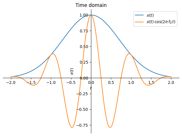
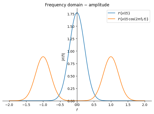
Amplitude modulation is relatively common in practice. We observe it, for example, when we measure the vibration of a plate with a laser and the laser’s base shakes; in the figures below, the displacement of the measured structure is denoted by \(x(t)\), while the laser’s base vibrates with \(\cos(2\pi\,f_0\,t)\).
By the way: amplitude modulation (AM) and frequency modulation (FM) are classic ways of transmitting information (e.g. a radio signal).
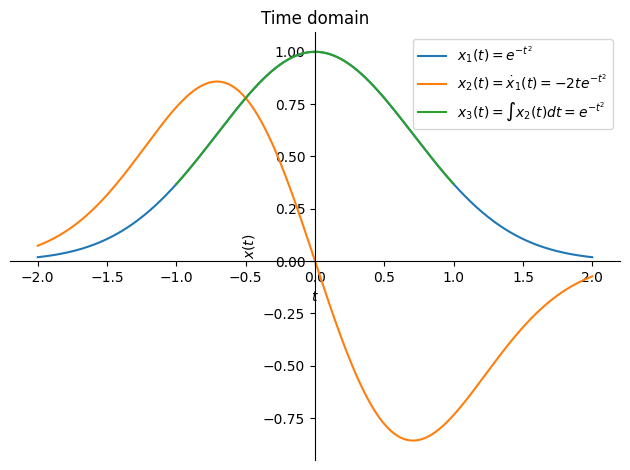
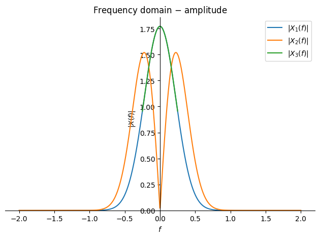
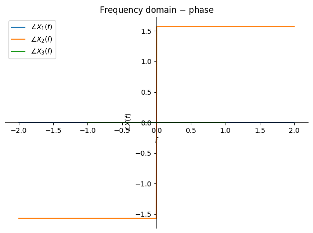
Differentiation#
Note
If \(\dot{x}(t)\) is the time derivative of \(x(t)\), their relation in the frequency domain is:
where it is assumed that \(x(t)\rightarrow 0\) as \(t\rightarrow \pm\infty\).
And the derivation:
import sympy as sym
t, f = sym.symbols('t, f', real=True)
x = sym.Function('x')
i = sym.I
π = sym.pi

X = sym.integrate(sym.diff(x(t),t)*sym.exp(-i*2*π*f*t), (t, -sym.oo, +sym.oo))
X
We must use integration by parts \(u = \mathrm{e}^{-\textrm{i}\,2\pi\,f\,t}\), \(\textrm{d}v= \dot{x}(t)\,\textrm{d}t\); we prepare \(\textrm{d}u\) and \(v\):
u = sym.exp(-i*2*π*f*t)
dv = sym.diff(x(t),t)

du = sym.diff(u, t)
v = sym.integrate(dv, t)
It follows that we must (the first part of integration by parts):
u*v
evaluate at the limits \(+\infty\) and \(-\infty\); according to the definition above, in both cases (because of the earlier assumption) \(x(t=\pm \infty)=0\).
Therefore only the second part of integration by parts remains:
sym.integrate(v*du, (t, -sym.oo, +sym.oo))
and with this we have completed the proof.
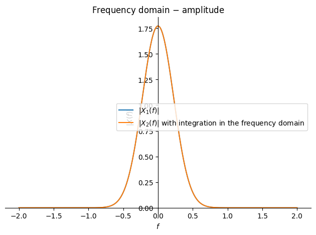
Integration#
Note
If \(\int_{-\infty}^t x(\tau)\,\textrm{d}\tau\) is the integral of the function \(x(t)\), their relation in the frequency domain is:
The derivation for integration follows from the one for differentiation:
where we make the substitution of the function: \(u(t)=\dot{x}(t)\) and \(\int_{-\infty}^t u(\tau)\,\textrm{d}\tau=x(t)\).
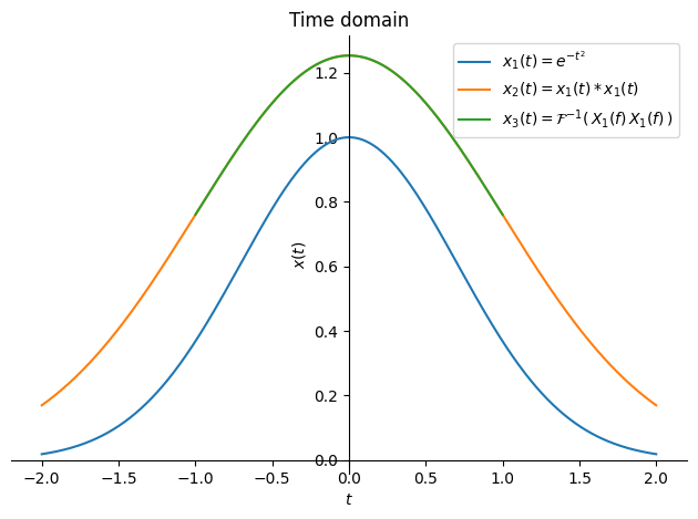
Differentiation and integration in the frequency domain are very important properties of the Fourier transform, since they allow us a simple transition between differentiated and integrated data.
Here it is worth emphasizing that time differentiation is an uncertain numerical operation, since it is based on a small difference of numbers (and the difference is then divided by a small number, which further increases the uncertainty). Differentiation in the frequency domain is not exposed to such uncertainty.
Furthermore, we emphasize that time integration is an unstable numerical operation, since the error of an individual step accumulates and therefore grows with time. Integration in the frequency domain is not exposed to such instability; it is true, however, that at the frequency 0 Hz we have an undefined result (division by 0).
Convolution of functions#
Note
The Fourier transform of the convolution of two functions is equal to the product of the Fourier transforms:
The symbol \(*\) denotes convolution:
We derive the above relation:
import sympy as sym
t, f, τ, v = sym.symbols('t, f, tau, v', real=True)
x = sym.Function('x')
y = sym.Function('y')
i = sym.I
π = sym.pi

X = sym.integrate(
        sym.integrate(x(τ)*y(t-τ)*sym.exp(-i*2*π*f*t), (τ, -sym.oo, +sym.oo)),
        (t, -sym.oo, +sym.oo))
X
We also introduce a new variable:
X = X.transform(t-τ, v)
X
Above, it is obvious that we can separate the integral over \(\tau\) and \(v\), and the separated integral represents the Fourier transforms \(X(f)\) and \(Y(f)\).
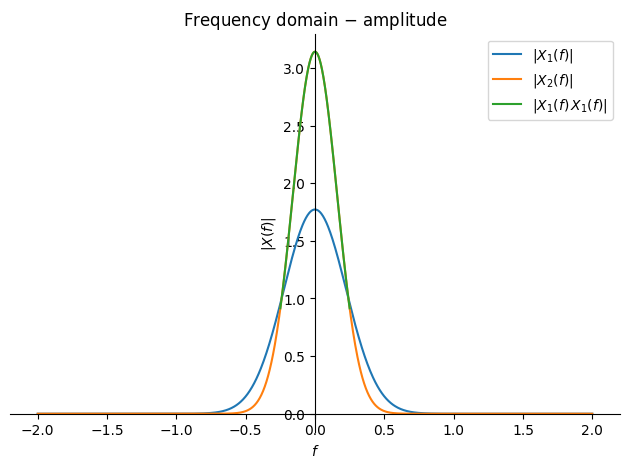
The Fourier transform of a convolution is perhaps the most useful property of the Fourier transform, since multiplication in the frequency domain significantly speeds up the computation of the convolution of two functions. We will make good use of this property in the discrete Fourier transform, while the simple example below shows the equivalence of the result in time versus the one in frequency.
Product of functions#
Note
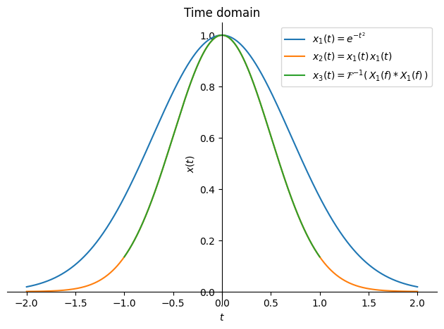
The Fourier transform of the product of two functions represents, in the frequency domain, the convolution of the Fourier transforms:
We derive the above relation:
Now we take into account \(\int_{-\infty}^{+\infty}\mathrm{e}^{\pm\textrm{i}\,2\pi\,a\,t}\,\textrm{d}t= \delta(a)\) (see Properties of the Dirac delta function) and prove the above derivation:
Below, let us look at a concrete example.
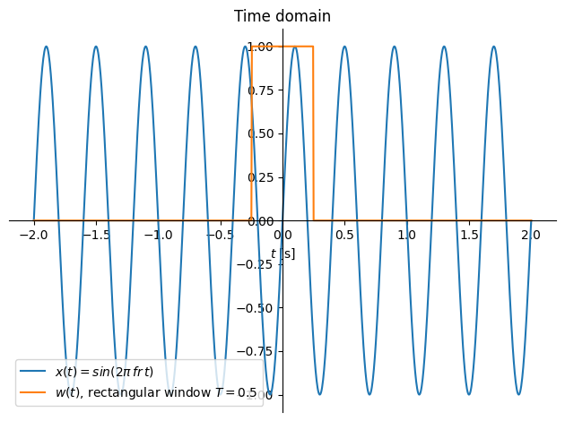
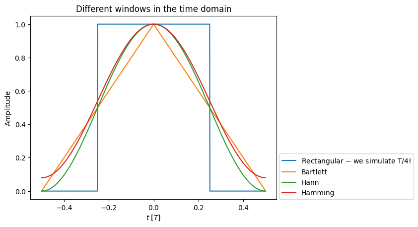
The use of windows#
Let us assume that we want to compute the Fourier transform of a deterministic signal \(x(t)\), which is in principle defined from \(-\infty\) to \(+\infty\), but which we observe only on the interval from \(-T/2\) to \(+T/2\). We obtain the following data:
where:
If we obtain the Fourier transform of \(x_T(t)\), then:
The message, then, is: \(X(f)\) represents the frequency transform of the function \(x(t)\), which we can observe only in a certain time-limited window \(w(t)\), and this window causes the Fourier transform to be distorted. We have already looked at the rectangular impulse \(w(t)\) above (Rectangular impulse) and found that its frequency transform is defined as:
where we used a notation that reveals the limit: as \(T\to 0\), \(W(0)=T\).
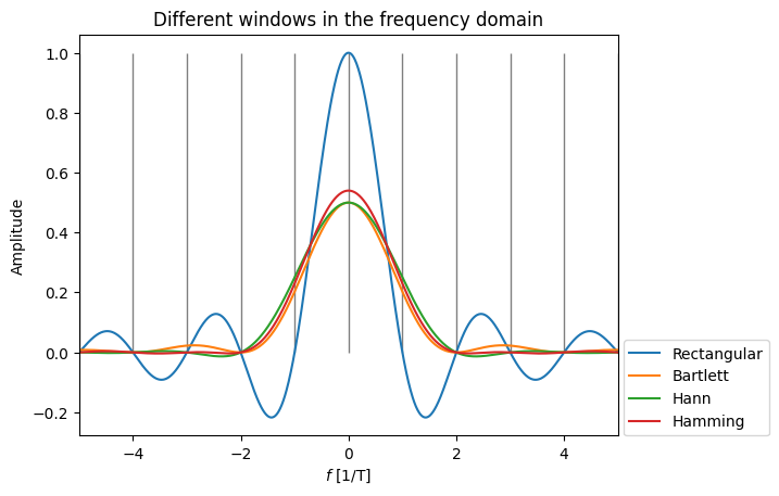
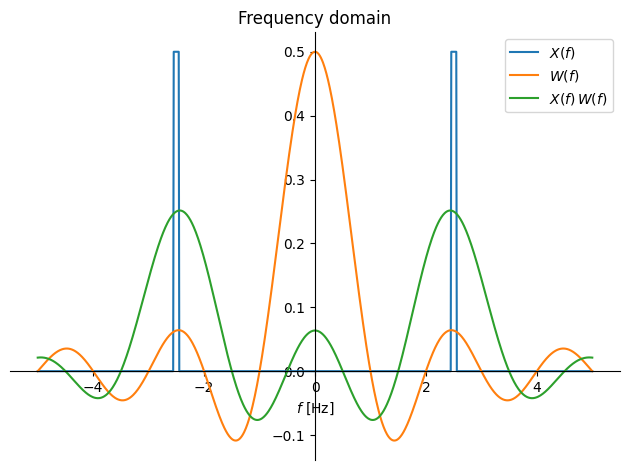
For a sinusoid of frequency fr with amplitude 1, we know that in the frequency domain it has amplitude 1/2 at the frequencies -fr and fr; on the other hand, above we defined the frequency function of the rectangular window. How the rectangular window distorts the sinusoid can be observed by convolving their frequency transforms (example below).