import numpy as np
from ipywidgets import interact
import matplotlib.pyplot as plt
%matplotlib inline
import sympy as sym
sym.init_printing()Introduction
Writing (a single) differential equation
Assume that a first-order differential equation can be written in explicit form:
where is a given function and .
Additionally, an initial condition is given:
The goal of solving the differential equation is to compute the function that solves the initial value problem defined above. Under certain conditions on the function , the initial value problem has a unique solution on an interval containing .
In numerical solving we always compute a table of the function that solves the given initial value problem. The nodes are usually equidistant:
and we call the (time) step (of integration).
Here we will look at some numerical methods for solving differential equations with an initial condition.
Euler’s method
The explicit Euler’s method is based on the Taylor series expansion of the function :
We make a method error of because we neglect the second and higher-order derivatives; now, given a known value and the derivative , we can estimate the value at the next time step . Once we know the values at , we repeat the procedure!
Steps of Euler’s method:
Set , , .
Compute the function value at :
and continue at step 2.
We solve the differential equation on the interval and . is the number of integration steps (how many times we perform step 2 in the algorithm above).
Numerical solution of the initial value problem:
at the values of the independent variable:
from IPython.display import YouTubeVideo
YouTubeVideo('cfZ8v0b-R8o', width=800, height=300)Error of Euler’s method
The error of Euler’s method at each step is of order .
Since over the interval from to we make this error times, the cumulative error is .
Locally the error is second order, but globally the error is first order, and because Euler’s method is so inaccurate, we rarely use it in practice!
Error estimate
The exact solution at step size is:
where is the numerical approximation and is the method error. Since the global error is first order, we can write the error as:
Similarly, for step size we can write:
where is the numerical approximation and is the method error:
Assuming that the constant is the same for step and step , we can determine the error estimate for the better approximation . Clearly:
then we determine the error estimate:
A note on the implicit Euler’s method
In the explicit Euler’s method we compute the solution at from the computed value at .
If the unknown value of the solution at , that is , appeared on the right-hand side as well, we would be talking about the implicit Euler’s method (or backward Euler’s method):
Because the sought value appears on both sides of the equation, to determine we must solve a (nonlinear) equation. The advantage of the implicit Euler’s method is that it is more stable (e.g., for stiff systems, which we will learn about later) than the explicit form, but it is numerically more demanding (because of solving the equation).
Numerical implementation
First we import the required libraries:
import numpy as np
import matplotlib.pylab as plt
%matplotlib inline
Next let us define Euler’s method:
def euler(f, t, y0, *args, **kwargs):
    """
    Euler's method for solving a system of differential equations: y' = f(t, y)

    :param f:  function returning the first derivative - f(t, y)
    :param t:  time vector where we compute the solution
    :param y0: initial value
    :param args: additional arguments of the function f (positional)
    :param kwargs: additional arguments of the function f (keyword)
    :return y: returns an np.array ``y`` of function values.
    """
    y = np.zeros_like(t)
    y[0] = y0
    h = t[1]-t[0]
    for i in range(len(t)-1):
        y[i+1] = y[i] + f(t[i], y[i], *args, **kwargs) * h
    return y
Let us prepare a function for the error estimate (in numerical terms it would be better to include the error estimate inside the euler function, but for clarity we present it separately):
def euler_error(f, t, y0, *args, **kwargs):
    """ Error estimate of Euler's method; the arguments are the same as for the `euler` function
    """
    n = len(t)
    if n < 5:
        raise Exception('There must be at least 5 nodes.')
    if n%2==0: # even number of nodes; remove one point and make it odd (so the number of subintervals is even)
        n = n - 1
    y_h = euler(f, t[:n], y0, *args, **kwargs)
    y_2h = euler(f, t[:n:2], y0, *args, **kwargs)
    E_h = y_h[-1] - y_2h[-1]
    return E_h
Numerical example
As an example, let us solve the differential equation that describes a falling body subjected to gravity and air resistance:
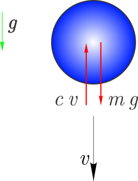
According to Newton’s second law, we can write the differential equation:
where is the mass, the gravitational acceleration, the air-resistance coefficient, and the velocity. We would like to solve the differential equation subject to the initial condition:
Let us define the right-hand-side function:
def f_air_resistance(t, y, g=9.81, m=1., c=0.5):
    return g-c*y/m
Let us define the initial condition and the time vector where we want the result:
v0 = 0
t = np.linspace(0, 10, 11)
t
array([ 0., 1., 2., 3., 4., 5., 6., 7., 8., 9., 10.])We call the euler function to compute the values of (velocity ):
y = euler(f_air_resistance, t, y0=v0)
y
array([ 0. , 9.81 , 14.715 , 17.1675 , 18.39375 ,
19.006875 , 19.3134375 , 19.46671875, 19.54335938, 19.58167969,
19.60083984])We plot the result:
plt.plot(t, y)
plt.title('Mass velocity as a function of time')
plt.xlabel('Time $t$ [s]')
plt.ylabel('Velocity $v$ [m/s]')
plt.show()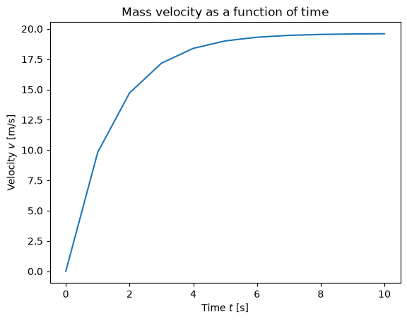
Let us now check the effect of the time step:
for n in [11, 101, 1001]:
    t = np.linspace(0, 10, n)
    y = euler(f_air_resistance, t, y0=v0, c=0.7)
    plt.plot(t, y, label=f'Time step: {t[1]:1.0e}')
plt.title('Mass velocity as a function of time')
plt.xlabel('Time $t$ [s]')
plt.ylabel('Velocity $v$ [m/s]')
plt.legend()
plt.show()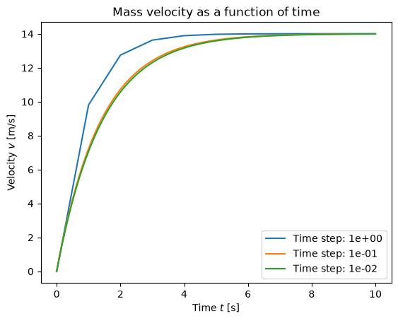
We observe that the numerical error decreases substantially when the step changes from 1 to 0.1!
Let us also estimate the error at 100 and 1000 subintervals:
n=101
t = np.linspace(0, 10, n)
euler_error(f_air_resistance, t, y0=v0)n=1001
t = np.linspace(0, 10, n)
euler_error(f_air_resistance, t, y0=v0)When we reduced the step to a tenth, the error decreased proportionally as well (first-order error).
Let us also look at the case where the air resistance c is an argument of the euler function and is passed via **kwargs to the f_air_resistance() function:
for c in np.linspace(0, 1, 5):
    t = np.linspace(0, 5, 1001)
    y = euler(f_air_resistance, t, y0=v0, c=c)
    plt.plot(t, y, label=f'$c={c}$')
plt.title('Mass velocity as a function of time for various air-resistance coefficients')
plt.xlabel('Time $t$ [s]')
plt.ylabel('Velocity $v$ [m/s]')
plt.legend()
plt.show()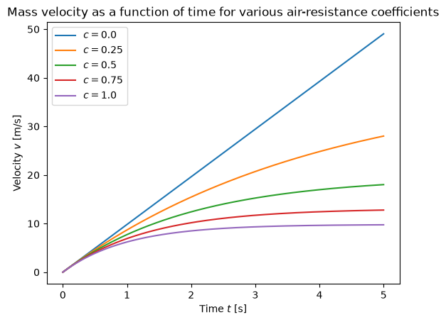
Second-order Runge–Kutta method
Euler’s method is first order (the global error is indeed first order). If we wanted to derive a second-order-error method, we would need to use the Taylor series expansion of , where we neglect the third and higher derivatives:
The local error of the method will thus be third order and the global error second order.
We use the substitutions and :
Because the right-hand side depends on both the independent variable and the dependent variable , we must use implicit differentiation:
We substitute into the Taylor series expression:
As can be seen from the expression above, we need additional derivatives. This poses a certain difficulty that can be avoided in various ways; in what follows we will look at the Runge–Kutta approach. Because we will need the expression above later, we have named it here .
Idea of the Runge–Kutta approach
The dilemma above is resolved by the Runge–Kutta method (developed in 1901) with an idea we have already encountered in Gaussian integration: it tries to find a more accurate solution with a weighted additional value of the function :
where , , , and are unknown constants (in principle from 0 up to and including 1). If we used in the expression above, we would derive a first-order method; but with an additional function value () it will turn out that we derive a second-order method.
We continue the search for the unknown constants , , , by writing in the form of a first-order Taylor series:
Now we substitute the derived back into the expression for :
We continue the derivation and rearrange the equation so that it resembles the one derived above with the Taylor series :
Now let us compare with the expression derived above:
We find that for equality to hold we must have:
So we have three equations and four unknowns. We can therefore choose one of the constants arbitrarily and compute the other three. If, for example, we choose , we would call this the modified Euler’s method and the remaining parameters would be: , . The choice of parameters has no essential effect on the solution. It is worth noting, however, that even the second-order Runge–Kutta method is rarely used, since better methods exist.
We substitute the parameters , , , and into the first equation of this section. Once the initial time and the initial condition are defined, we use the second-order Runge–Kutta method:
Fourth-order Runge–Kutta method
Similarly to how we derived the second-order Runge–Kutta method, the fourth-order Runge–Kutta method is derived. For the fourth-order method, too, there are several variants, and by the fourth-order Runge–Kutta method we mean the following method:
The steps of the fourth-order Runge–Kutta method are:
Set and , ,
Compute the coefficients: , , , ,
Compute the value of the solution of the differential equation at :
and continue at step 2.
Error of the fourth-order Runge–Kutta method
The fourth-order Runge–Kutta method is named so because it has a local error of fifth order , but we make this error times, so the global error is fourth order .
Error estimate
The exact result at step size is:
where is the numerical approximation of the solution and is the method error. Since the global error is fourth order, we can write the error as:
Similarly, for step size we can write:
where is the numerical approximation of the solution and is the method error:
Assuming that the constant is the same for step and step , we can compute the error estimate for the better approximation .
First, it is true that:
Numerical implementation
def runge_kutta_4(f, t, y0, *args, **kwargs):
    """
    Fourth-order Runge–Kutta method for solving a differential equation: y' = f(t, y)

    :param f: function called with the parameters t and y, returning
              the value of the first derivative
    :param t: equidistant time vector, i.e., the independent variable
    :param y0: initial value
    :param args: additional arguments of the function f (positional)
    :param kwargs: additional arguments of the function f (keyword)
    :return y: function values.
    """
    def RK4(f, t, y, *args, **kwargs):
        k0 = h*f(t, y, *args, **kwargs)
        k1 = h*f(t + h/2.0, y + k0/2.0, *args, **kwargs)
        k2 = h*f(t + h/2.0, y + k1/2.0, *args, **kwargs)
        k3 = h*f(t + h, y + k2, *args, **kwargs)
        return (k0 + 2.0*k1 + 2.0*k2 + k3)/6.0

    y = np.zeros_like(t)
    y[0] = y0
    h = t[1]-t[0]

    for i, ti in enumerate(t[:-1]):
        y[i+1] = y[i] + RK4(f, ti, y[i], *args, **kwargs)

    return y
Function for the error estimate:
def runge_kutta_4_error(f, t, y0, *args, **kwargs):
    """ Error estimate of the fourth-order Runge–Kutta method; arguments are the same as for `runge_kutta_4`
    """
    n = len(t)
    if n < 5:
        raise Exception('There must be at least 5 nodes.')
    if n%2==0: # even number of nodes; remove one point and make it odd (so the number of subintervals is even)
        n = n - 1
    y_h = runge_kutta_4(f, t[:n], y0, *args, **kwargs)
    y_2h = runge_kutta_4(f, t[:n:2], y0, *args, **kwargs)
    E_h = (y_h[-1] - y_2h[-1])/15
    return E_h
Numerical example
Let us now look at the example of computing the velocity of a falling mass:
def f_air_resistance(t, y, g=9.81, m=1., c=0.5):
    return g-c*y/m
Let us provide the initial condition and the time vector where we want the result:
v0 = 0
t = np.linspace(0, 10, 11)
t
array([ 0., 1., 2., 3., 4., 5., 6., 7., 8., 9., 10.])For comparison, let us compute the solution with the euler and runge_kutta_4 functions:
y_euler = euler(f_air_resistance, t, y0=v0, c=0.4)
y_rk4 = runge_kutta_4(f_air_resistance, t, y0=v0, c=0.4)
We plot the result:
plt.plot(t, y_euler, label='Euler')
plt.plot(t, y_rk4, label='RK4')
plt.title('Mass velocity as a function of time')
plt.xlabel('Time $t$ [s]')
plt.ylabel('Velocity $v$ [m/s]')
plt.legend()
plt.show()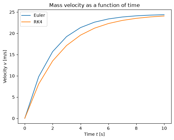
Let us also look at the numerical error:
n=101
t = np.linspace(0, 10, n)
runge_kutta_4_error(f_air_resistance, t, y0=v0, c=0.4)n=1001
t = np.linspace(0, 10, n)
runge_kutta_4_error(f_air_resistance, t, y0=v0, c=0.4)When the step is reduced to a tenth, the error decreased by about 104 times (which matches the expectation for a fourth-order method).
Using scipy to solve ordinary differential equations
The scipy package has many numerical methods implemented for solving initial value problems of ordinary differential equations. Here we will look at the function scipy.integrate.solve_ivp, which is suitable for most initial value problems.
scipy.integrate.solve_ivp
Syntax for use (IVP - Initial Value Problem):
scipy.integrate.solve_ivp(fun, t_span, y0, method='RK45',
                          t_eval=None, dense_output=False,
                          events=None, vectorized=False,
                          args=None, **options)
An explanation of all the arguments is in the documentation; here we will highlight a few:
funis the right-hand side (func(t, y...)),t_spana tuple (t0,tf) defining the initial timet0and final timetf,y0a list of initial value(s),methoddefines the numerical method (the default is the explicit ‘RK45’; for stiff systems the following are better: ‘Radau’, ‘BDF’, ‘LSODA’),t_evalis used if we want the solution at specific values of the independent variable,dense_outputwhether a continuous solution is also prepared, defaultFalse,eventsfor tracking events that stop solving the initial value problem (e.g., when the mass touches the ground and the relative distance to the ground is zero).argsfor passing arguments into the functionfun(see the example below).
The result of calling solve_ivp is an object with attributes (selected):
tthe values of the independent variable at which the result is computed,ythe result,solthe continuous-solution function (only in the case ofdense_output=True)successisTrueif the solution was computed successfully or terminated due to an event (events).
Numerical example
Let us define the initial condition and the time vector where we want the result (we show only the first ten elements):
v0 = 0
t = np.linspace(0, 10, 101)
t[:10]
array([0. , 0.1, 0.2, 0.3, 0.4, 0.5, 0.6, 0.7, 0.8, 0.9])We pass the arguments (g=9.81, m=1., c=0.4) into the function via the args parameter:
from scipy.integrate import solve_ivp
y_ivp = solve_ivp(f_air_resistance, t_span=(t[0], t[-1]), y0=[v0], args=(9.81, 1, 0.4))
We could also use a lambda expression (documentation):
y_ivp = solve_ivp(lambda t,y: f_air_resistance(t, y, c=0.4), t_span=(t[0], t[-1]), y0=[v0])The lambda expression used above, lambda t, y: f_air_resistance(t, y, c=0.4), is equivalent to:
def function_name(t, y):
    return f_air_resistance(t, y, c=0.4)
Let us look at the result:
y_ivp message: The solver successfully reached the end of the integration interval.
success: True
status: 0
t: [ 0.000e+00 1.000e-04 1.100e-03 1.110e-02 1.111e-01
1.111e+00 2.982e+00 5.236e+00 7.948e+00 1.000e+01]
y: [[ 0.000e+00 9.810e-04 1.079e-02 1.086e-01 1.066e+00
8.800e+00 1.708e+01 2.150e+01 2.350e+01 2.407e+01]]
sol: None
t_events: None
y_events: None
nfev: 56
njev: 0
nlu: 0Because solve_ivp is already set up for a system of first-order ordinary differential equations, the result is given in two dimensions. The sought result is therefore: y_ivp.y[0].
For comparison, here is also the result with our own fourth-order Runge–Kutta implementation:
y_rk4 = runge_kutta_4(f_air_resistance, t, y0=v0, c=0.4)y_rk4[:10]array([0. , 0.96163898, 1.88557156, 2.77327623, 3.6261735 ,
4.44562819, 5.23295161, 5.98940363, 6.71619474, 7.41448797])We plot the result:
plt.plot(y_ivp.t, y_ivp.y[0], '.', label='solve_ivp')
plt.plot(t, y_rk4, label='RK4')
plt.title('Mass velocity as a function of time')
plt.xlabel('Time $t$ [s]')
plt.ylabel('Velocity $v$ [m/s]')
plt.legend()
plt.show()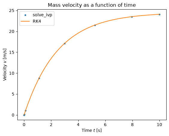
System of ordinary differential equations
Above we looked at solving the initial value problem of a single ordinary differential equation; now we will generalize the solving to an initial value problem for a system of first-order ordinary differential equations.
Such a system is written as:
where additional (initial) conditions are given:
By we denote the independent variable (it need not always be time) and by the vector of right-hand sides.
We compute the solution of a system of differential equations at , that is function values at each step , and . It can be proved that any method we derived for first-order differential equations can also be used for a system of first-order ordinary differential equations if we replace the scalar quantities with the corresponding vector ones.
Numerical implementation
The Euler and fourth-order Runge–Kutta methods need only minor adjustments (y0 is a numerical array, f returns a list of derivative values):
def euler_system(f, t, y0, *args, **kwargs):
    """
    Euler's method for solving a system of first-order ordinary differential equations: y' = f(t, y)

    :param f:  function called with the parameters t and y, returning a list
               of right-hand-side functions
    :param t:  equidistant (time) vector of the independent variable
    :param y0: list of initial values
    :param args: additional arguments of the function f (positional)
    :param kwargs: additional arguments of the function f (keyword)
    :return y: returns an np.array ``y`` of function values.
    """
    y = np.zeros((t.shape[0], len(y0)))
    y[0] = np.copy(y0)
    h = t[1]-t[0]
    for i, ti in enumerate(t[:-1]):
        # here is the essence of Euler's method
        y[i+1] = y[i]+f(ti, y[i], *args, **kwargs)*h
    return y
def runge_kutta_4_system(f, t, y0, *args, **kwargs):
"""
Fourth-order Runge–Kutta method for solving a system of first-order ordinary differential equations: y' = f(t, y)
:param f: function called with the parameters t and y, returning a list
of right-hand-side functions
:param t: equidistant (time) vector of the independent variable
:param y0: list of initial values
:param args: additional arguments of the function f (positional)
:param kwargs: additional arguments of the function f (keyword)
:return y: returns an np.array ``y`` of function values.
"""
def RK4(f, t, y, *args, **kwargs):
k0 = h*f(t, y, *args, **kwargs)
k1 = h*f(t + h/2.0, y + k0/2.0, *args, **kwargs)
k2 = h*f(t + h/2.0, y + k1/2.0, *args, **kwargs)
k3 = h*f(t + h, y + k2, *args, **kwargs)
return (k0 + 2.0*k1 + 2.0*k2 + k3)/6.0
y = np.zeros((t.shape[0], len(y0)))
y[0] = np.copy(y0)
h = t[1]-t[0]
for i, ti in enumerate(t[:-1]):
y[i+1] = y[i] + RK4(f, ti, y[i], *args, **kwargs)
return yNumerical example
We extend the falling mass to planar motion; let the magnitude of the air-resistance force be defined as:
The air-resistance force acts in the opposite direction to the velocity vector.
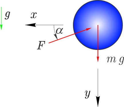
With the help of the figure, we define the force in the direction:
Similarly, the force in the direction is:
According to Newton’s second law, we write a system of two (coupled) first-order differential equations:
is the mass, the gravitational acceleration, the air-resistance coefficient, and and the velocities in the and directions, respectively. We would like to solve the differential equation subject to the initial condition:
Let us define the list of right-hand sides:
def f_air_resistance_force(t, y,  g=9.81, m=1., c=0.5):
    vx, vy = y
    return np.array([-c*vx*np.sqrt(vx**2+vy**2)/m, g-c*vy*np.sqrt(vx**2+vy**2)/m])
Let us define the initial condition and the time vector where we want the result:
y0 = np.array([5., 5.])
t = np.linspace(0, 5, 101)
t[:5]
array([0. , 0.05, 0.1 , 0.15, 0.2 ])For comparison, let us compute the solution with the runge_kutta_4 and solve_ivp functions:
y_RK4 = runge_kutta_4_system(f_air_resistance_force, t=t, y0=y0)
y_ivp = solve_ivp(f_air_resistance_force, t_span=(t[0], t[-1]), y0=y0, t_eval=t)
Let us look at the result:
y_ivp.y[:,:5]array([[5. , 4.23209907, 3.63858619, 3.16619484, 2.78087608],
[5. , 4.68459713, 4.48359747, 4.35932897, 4.28742151]])y_RK4[:5].Tarray([[5. , 4.23211316, 3.6399137 , 3.16660748, 2.77780226],
[5. , 4.68462761, 4.48494405, 4.35999931, 4.28466858]])We plot the result:
plt.plot(t, y_ivp.y[0], label='$v_x$')
plt.plot(t, y_ivp.y[1], label='$v_y$')
plt.title('Mass velocity (resistance and force) as a function of time')
plt.xlabel('Time $t$ [s]')
plt.ylabel('Velocity $v$ [m/s]')
plt.legend()
plt.show()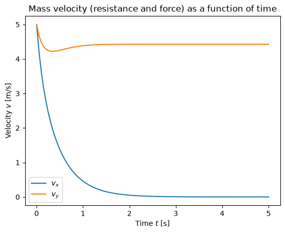
Reformulating a higher-order differential equation into a system of first-order differential equations
We will look at how an ordinary differential equation of arbitrary order :
with initial conditions:
is reformulated into a system of first-order differential equations.
First, instead of derivatives we introduce new variables:
The th-order differential equation written with the new variables is:
We have obtained a system of first-order ordinary differential equations:
with initial conditions:
Numerical example
We return to the falling mass:
But this time let us write Newton’s second law in terms of displacement (a second-order differential equation):
is the mass, the gravitational acceleration, the air-resistance coefficient, and and the acceleration in the chosen coordinate system. Initial conditions:
We have a system of two second-order differential equations. By introducing new variables :
We prepare the system of first-order differential equations:
Let us define the Python function of right-hand sides / first derivatives:
def f_air_resistance_coupled(t, y, g=9.81, m=1., c=0.5):
    x, vx, y, vy = y
    return np.array([vx, -c*vx*np.sqrt(vx**2+vy**2)/m, vy, g-c*vy*np.sqrt(vx**2+vy**2)/m])
Let us define the initial condition and the time vector where we want the result:
y0 = np.array([0., 5., 0., 5.])
t = np.linspace(0, 5, 101)
t[:5]
array([0. , 0.05, 0.1 , 0.15, 0.2 ])We compute the solution:
y_ivp = solve_ivp(f_air_resistance_coupled, t_span=(t[0], t[-1]), y0=y0, t_eval=t)Let us look at the result ():
y_ivp.y[:,:5]array([[0. , 0.22992477, 0.42611996, 0.59587483, 0.74424286],
[5. , 4.23183658, 3.64002431, 3.16703014, 2.77775353],
[0. , 0.24153615, 0.47038377, 0.69124852, 0.9072755 ],
[5. , 4.68435696, 4.48497294, 4.36034218, 4.28444004]])We plot the results; first the velocity, then the position (the coordinate is positive downward)!
plt.plot(t, y_ivp.y[1], label='$v_x$')
plt.plot(t, y_ivp.y[3], label='$v_y$')
plt.title('Mass velocity as a function of time')
plt.xlabel('Time $t$ [s]')
plt.ylabel('Velocity [m/s]')
plt.legend()
plt.show()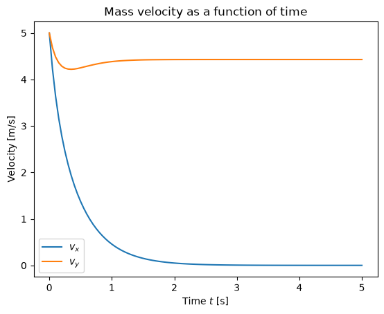
plt.scatter(y_ivp.y[0], y_ivp.y[2], marker='.')
plt.xlabel('$x$ [m]')
plt.ylabel('$y$ [m]')
plt.title('Mass position')
plt.show()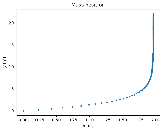
Stability of solving differential equations*
The numerical solution of differential equations is subject to method error and round-off error. These errors differ for different numerical methods.
Solving a differential equation is stable if a small change in the initial condition leads to a small change in the computed solution; otherwise we speak of instability of the solution.
Stability depends on the differential equation, on the numerical method used, and on the integration step .
Example of a simple oscillator
Let us first look at an example of solving the differential equation of a simple oscillator.
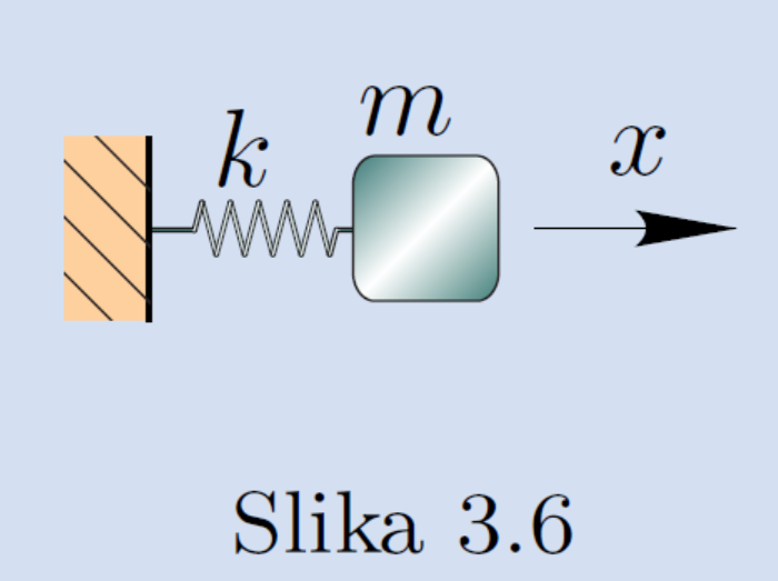
The figure (source: Slavič, Dinamika, mehanska nihanja in mehanika tekočin, 2017) shows a dynamic system (mass , stiffness ) whose differential equation is
We reformulate this differential equation into the standard form of free vibration:
where the natural angular frequency is:
and we expect a response of the form:
Numerical example
First let us define the vector of initial conditions and the function of right-hand sides / first derivatives (we convert the second-order differential equation into a system of first-order differential equations ), where :
def f_oscillator(t, y, omega0=2*np.pi):
    """
    Right-hand-side function for an oscillator with one degree of freedom

    :param t: time
    :param y: list of initial values
    :param omega: natural angular frequency
    :return y': list of derivative values
    """
    return np.array([y[1], -omega0**2*y[0]])
Let us define the data and the analytical solution:
x0 = 1.
omega0 = 2*np.pi
x_initial_conditions = np.array([x0, 0.])
t1 = 4.
time = np.linspace(0, t1, 500)
displacement = x0*np.cos(omega0*time) # analytical solution
velocity = -x0*omega0*np.sin(omega0*time) # analytical solution
Solution using the Euler and fourth-order Runge–Kutta methods:
t_Eu = np.linspace(0, t1, 101)
t_RK4 = t_Eu
dt = t_Eu[1]

x_Eu = euler_system(f_oscillator, t_Eu, x_initial_conditions)
x_RK4 = solve_ivp(f_oscillator, t_span=(t_RK4[0], t_RK4[-1]), y0=x_initial_conditions, t_eval=t_RK4).y
Let us plot the results:
plt.plot(time, displacement, label='Analytical solution')
plt.plot(t_Eu, x_Eu[:,0], '.', label='Euler')
plt.plot(t_RK4, x_RK4[0], '.', label='Runge-Kutta 4')
plt.legend()
plt.title('Stability of different methods')
plt.ylabel('Displacement [m]')
plt.xlabel('Time [s]')
plt.show()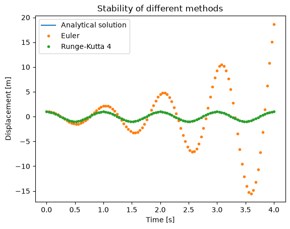
We observe that Euler’s method is unstable, and if we increased the step, the fourth-order Runge–Kutta method would also become unstable.
Why is Euler’s method so unstable?
x_Eu[:10,0]array([ 1. , 1. , 0.93683453, 0.8105036 , 0.62499707,
0.3882947 , 0.1121141 , -0.18859332, -0.49638247, -0.79225904])Let us recall Euler’s method:
which tells us that we determine the displacement from the position and the velocity . The initial conditions stem from the maximum deflection , and at that point the velocity is , which means that . Already in the first step we therefore make a relatively large error. But why does the value then start to grow in an alternating fashion?
Recall that the analytical solution is , and therefore .
We substitute the prepared expressions into Euler’s method and rearrange:
Assume we look at the state at a time , when and :
If the absolute value of the expression is greater than 1, then at time the value will be greater than in the previous step, and probably again in the next one. It follows that instability can occur. To avoid it, the following must hold:
Note: in some books you will also see the value ; a unique bound for all differential equations cannot be defined; in general, however, the step is defined relative to the shortest period in the differential equation (e.g.: is essentially the same as , i.e., ). The period is defined relative to the highest natural frequency of the system , which we compute from the eigenvalue of the system.
Additional: Example of the Van der Pol oscillator
The purpose of this example is to show how the choice of integrator can affect the speed of solving a problem! The Van der Pol oscillator is described here.
Let us define the list of derivatives:
def f_van_der_pol(t, y, mu=1000):
    """
    Right-hand-side function for the Van der Pol oscillator

    :param t: time
    :param y: list of initial values
    :param mu: damping and nonlinearity parameter
    :return y': list of derivative values
    """
    return np.array([y[1], mu*(1-y[0]**2)*y[1]-y[0]])
x_initial_conditions = np.array([1.5, 0.])
dt = 0.1
t1 = 3000Solution using the RK45 method (this is an explicit scheme, which is not suitable for stiff systems of differential equations; solving is very slow, so we compute the solution only up to t1/100):
vp_RK45 = solve_ivp(f_van_der_pol, t_span=(0., t1/100), y0=x_initial_conditions, method='RK45')The implicit BDF scheme (Backward Differentiation Formulas) turns out here to be much more suitable. Because of its stability, the steps can be much larger and therefore the solving is much faster:
vp_BDF = solve_ivp(f_van_der_pol, t_span=(0., t1), y0=x_initial_conditions, method='BDF')plt.plot(vp_BDF.t, vp_BDF.y[0], 'C1.', label='Displacement - BDF [m]')
plt.plot(vp_RK45.t, vp_RK45.y[0], 'C0.', label='Displacement - RK45 [m]')
plt.xlabel('Time [s]')
plt.legend(loc=(1.01, 0));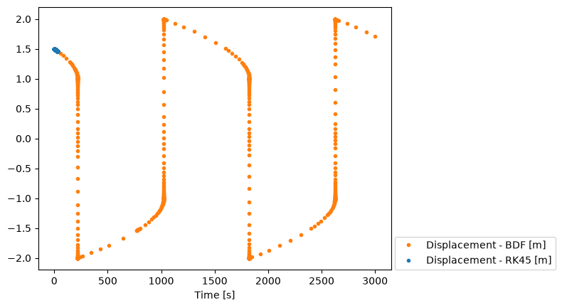
Additional: symbolic solving of a second-order differential equation
We will look at the example shown in the figure, where a mass is on an incline of slope . The coefficient of friction is , and the gravitational acceleration is . The initial velocity is , the displacement .
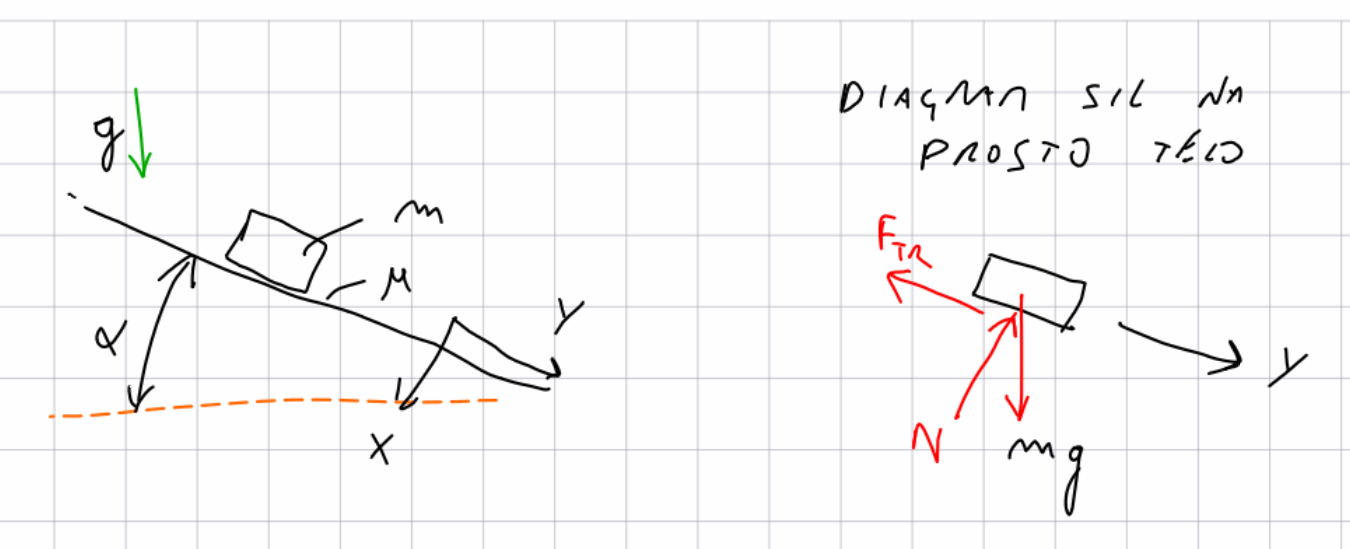 The equation of motion (only for the direction) is defined according to Newton’s second law (see the free-body force diagram).
Derivation of the equation of motion
y = sym.Function('y')
m, mu, g, alpha, t, v0 = sym.symbols('m, mu, g, alpha, t, v0')
eq = sym.Eq(m*y(t).diff(t,2),  m*g*sym.sin(alpha)-m*g*sym.cos(alpha)*mu)
eqThe solution of the equation is:
dsol = sym.dsolve(eq, y(t))
dsolTo determine and , we substitute :
dsol.args[1].subs(t, 0)Then we differentiate with respect to time and again substitute :
dsol.args[1].diff(t).subs(t, 0)Based on the initial conditions, we have therefore determined the constants:
initial_conditions = {'C1': 0, 'C2': v0}The solution follows:
solution = dsol.args[1].subs(initial_conditions)
solutionLet us prepare functions for the numerical call:
data = {mu: 0.3, alpha: 15*np.pi/180, v0: 1., g: 9.81} # here we use np.pi so that we have a numerical value

displacement = sym.lambdify(t, solution.subs(data), 'numpy')
velocity = sym.lambdify(t, solution.diff(t).subs(data), 'numpy')

print('Displacement at 0s: {:g}m'.format(displacement(0)))
print('Velocity at 0s: {:g}m/s'.format(velocity(0)))
Displacement at 0s: 0m
Velocity at 0s: 1m/s
Let us prepare the plot:
time = np.linspace(0, 4, 100)
time2 = np.linspace(0, 4, 5)
def figure():
plt.plot(time, displacement(time), 'C0', label='Displacement [m]')
plt.plot(time, velocity(time), 'C1', label='Velocity [m/s]')
plt.plot(time2, displacement(time2), 'C0o', label='Displacement - large step [m]')
plt.plot(time2, velocity(time2), 'C1o', label='Velocity - large step [m/s]')
plt.xlabel('Time [s]')
plt.ylabel('Displacement [m] / Velocity [m/s]')
plt.legend(loc=(1.01, 0));
plt.show()figure()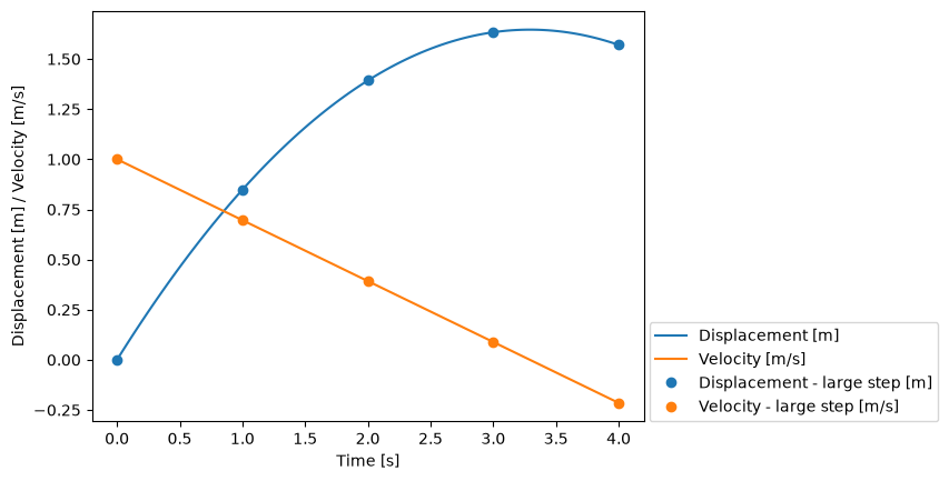
Symbolic reformulation of the differential equation into a system of first-order differential equations
Let us recall the original differential equation:
eqLet us define new variables and prepare the function :
y0 = sym.Function('y0')
y1 = sym.Function('y1')
f = sym.simplify(eq.args[1]/m)
fNow let us connect the new variables.
Let be equal to :
eq1 = sym.Eq(y0(t).diff(t), y1(t))
eq1Let the derivative (which is essentially ) be equal to the function :
eq2 = sym.Eq(y1(t).diff(t), f)
eq2We write the expressions above in vector form:
y_derivative = [y0(t).diff(t), y1(t).diff(t)]
y_derivativef_vec = [y1(t), f]
f_vecLet us now recall f_vec:
f_vecIf we solve numerically, then we write the function as:
acceleration = float((eq.args[1]/m).simplify().subs(data))
acceleration # investigate why we defined it this way here! hint: type(acceleration)def F_block(t, y):
return np.array([y[1], acceleration],dtype=float)Let us check the function at the initial time s and at the initial conditions :
y_initial_conditions = np.array([0, data[v0]])
y_initial_conditions
array([0., 1.])F_block(0., y_initial_conditions)array([ 1. , -0.30370487])Now let us use Euler’s method:
#%%timeit
x_Eu = np.linspace(0, 4, 5)
y_Eu = euler_system(F_block, x_Eu, np.array([0, 1.]))
y_Eu
array([[ 0. , 1. ],
[ 1. , 0.69629513],
[ 1.69629513, 0.39259025],
[ 2.08888538, 0.08888538],
[ 2.17777075, -0.2148195 ]])We plot and compare with the analytical solution:
def plot_euler(n=5):
    x_Eu = np.linspace(0, 4, n)
    y_Eu = euler_system(F_block, x_Eu, np.array([0, 1.]))
    plt.title('Euler\'s method with step $h={:g}$'.format(x_Eu[1]-x_Eu[0]))
    plt.plot(time, displacement(time), 'C0', label='Displacement - analytical [m]')
    plt.plot(time, velocity(time), 'C1', label='Velocity - analytical [m/s]')
    plt.plot(x_Eu, y_Eu[:, 0], 'C0.', label='Displacement - Euler [m]')
    plt.plot(x_Eu, y_Eu[:, 1], 'C1.', label='Velocity - Euler [m/s]')
    plt.xlabel('Time [s]')
    plt.ylabel('Displacement [m] / Velocity [m/s]')
    plt.ylim(-0.5, 2.5)
    plt.legend(loc=(1.01, 0))
    plt.show();
interact(plot_euler, n=(3, 10, 1));