Object-oriented programming, symbolic computation

Object-oriented programming¶

In programming there are various approaches; the Python documentation (docs.python.org) mentions, for example:

1. procedural: a list of instructions on what to do (e.g.: C, Pascal)

2. declarative: we describe what we want, and the programming language carries it out (e.g.: SQL)

3. functional: programming based on functions (e.g.: Haskell )

4. object-oriented: the program is based on objects that have properties, functions, ... (e.g.: Java, Smalltalk)

Python is an object-oriented programming language, but it does not force us to use objects in every case. As we will see later, object-oriented programming has many advantages, but it can often be cumbersome and would make a program unnecessarily complex. For this reason, we avoid explicit object-oriented programming whenever possible.

Object-oriented programming in Python is based on classes, and objects are instances of a class. We will look at only some of the basics of object-oriented programming (so that you can more easily understand the code of other authors and adapt it to your own needs).

A class is defined with the class statement (documentation):

class ClassName:
    '''docstring'''
    [expression 1]
    [expression 2]
    .
    .

where the class name (i.e., ClassName) is, per PEP8, written with a capital first letter. If the name consists of several words, each one is capitalized (the so-called CamelCase convention).

Let’s look at an example:

Before we go into the details of understanding the code, let’s create an instance of the class (i.e., an object):

Functions defined inside a class are called methods when we call them on objects.

In the example above, we use the area method like this:

The name self is a reference to the instance of the class (the object that will be created). Names defined inside the class become attributes of the object.

An example of the height attribute:

Where does the result 1 come from? When we create an object, the initialization function __init__() runs first; its arguments are the arguments we pass to the class.

Example:

We have also prepared a method that changes the width attribute:

We can also change attributes directly, but we usually avoid this (because of the possibility of errors and misuse).

Example:

Inheritance¶

An important property of classes is inheritance; the name itself says it all: just as we humans inherit from our parents, the same holds for classes. Each class (class) can thus inherit the properties of some other class (documentation). It can even have several parents (we will not go into these details here).

The syntax of a class that inherits is:

class Child(Parent):
    [expression]
    .
    .

Note: even if we do not define a parent for a class, the class inherits from object.

An example where the new class Square inherits from an existing one (Rectangle):

Now let’s look at how it is used:

The Square class does not define a method for computing the area, but it inherited it from the Rectangle class, and therefore has a method for computing the area:

If we change the width, the area changes accordingly:

Example of inheriting from the list class¶

First we prepare a list:

If we want to add a value to the list, we use the append method (this is a method that objects of type list have):

Then we plot the list (first we import matplotlib):

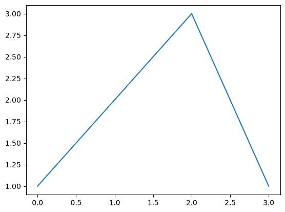
If we do something like this often, then it is better to prepare our own List class that inherits from list and add a method draw for plotting:

An instance of the object is:

Although we did not define the append method, the new class inherited it from the list class:

It also has a method for plotting:

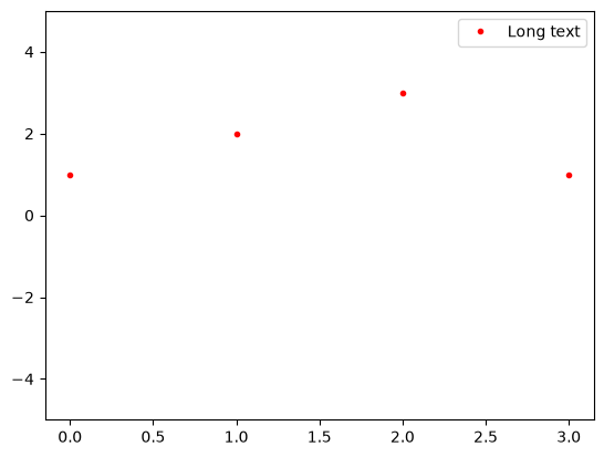
Symbolic computation with SymPy¶

The term symbolic computation means that we solve mathematical expressions by machine in the form of abstract symbols (and not numerically). Machine symbolic computation helps us when we are interested in the result in symbolic form and the expressions are too large to solve by hand on paper. We also resort to machine solving to reduce the chance of error (in extensive computations people can make mistakes).

Symbolic computation is by no means a substitute for numerical methods!

We will look at some of the basics; some recommended additional resources are:

• J.R. Johansson Scientific python lectures,

• SymPy - the official documentation of the module,

• An excellent article by some of the SymPy authors: Meurer et. al, 2017.

SymPy is one of the computer algebra systems (CAS), which, in addition to its capabilities, has the advantage of being written entirely in Python (the alternative Python package Sage, for example, is not written entirely in Python).

Some dedicated commercial tools:

• Mathematica

• Maple

First we import the SymPy module; typically the package is imported as sym:

You may notice that SymPy is also imported with from sympy import *. As a rule, we avoid this, since it unnecessarily fills the program’s base namespace with SymPy names. In the latter case, the package’s functions (e.g., sympy.Sum) are accessed directly (e.g., Sum), which can be appealing but starts to bother us when we add other packages (e.g., numpy), which, in addition to confusion, can lead to functions with the same name being “overwritten”.

In order to get nicely formatted LaTeX output, we use:

Defining variables and numerical computation¶

We define variables like this:

We can check the type:

We notice that the variable x is now a Symbol from the sympy package.

Now we can make a simple computation:

We can also name a function; here is an example where we use the sine function and the constant $\pi$:

The reader may be wondering why we need a new function sympy.sin(), since we already have the one from the numpy package! The reason is that symbolic computation requires a completely different treatment than numerical computation, and therefore the code behind it is entirely different.

If we want to write an equation, i.e., to equate one expression to another, we do it like this:

Undefined mathematical functions are written as (documentation):

Now we can, for example, define a differential equation:

When defining variables, we can add assumptions:

The assumptions are then taken into account in the computation. In general, we know that $\sqrt{(x^2)}\ne x$, but if $x$ is positive, then $\sqrt{(x^2)}= x$, and sympy, given the assumptions, computes the correct result:

With the assumptions0 method we look at an object’s assumptions:

SymPy knows the types of numbers (documentation):

• Float real numbers (floating point, arbitrary precision),

• Rational rational numbers,

• Integer integers,

• complex numbers are written with the imaginary unit I (e.g., 2 + 3*sym.I).

These types are important, as they can affect the way of solving and the solution.

Rational numbers¶

Above we have already defined real numbers. Let’s now look at rational numbers with an example:

Some computations:

Complex numbers¶

The imaginary number is written with I (this is different from numpy, where the imaginary part is defined with j):

Numerical computation¶

In symbolic computation we first solve analytical expressions, simplify them, etc., and then we often also want to compute a concrete result.

Let’s look at an example:

If we now want to use a value instead of $x$, e.g., 0.5, we do it with the subs() method (documentation):

Above we used the constant $\pi$ (documentation); some commonly used constants are:

• sympy.pi for the number $\pi$,

• sympy.E for the natural number $e$,

• sympy.oo for infinity.

As we saw above, subs() performs the substitution and then the simplifications that are obvious; it did not compute the number $\pi$ as a real (decimal) number. We must explicitly request this with the method:

• evalf (evaluate function, documentation) or

• N,

both of which have the argument n (number of digits).

Let’s look at an example:

It is similar with N:

In passing, we have shown that, provided the expression contains no floating-point numbers, we can display the result to arbitrary precision (documentation).

In the subs function we can also use a dictionary. Example:

or a list of tuples:

Similarly, the sympy.evalf() method has a subs argument that accepts a dictionary of substitutions, for example:

The sympy.subs method can also replace a symbol (or expression) with another expression:

SymPy and NumPy¶

We often connect sympy with numpy. As an example, let’s look at how we would compute the expression:

efficiently and numerically at a thousand values of $x$.

First we import the numpy package:

We prepare a numerical array of values:

Based on what is written above and our prior knowledge, we use a list comprehension:

We notice that this is slow, so let’s measure the time required:

Using the lambdify function¶

A significantly faster approach is to use the lambdify approach, where a compiled function is prepared, optimized for numerical execution. The syntax of the sympy.lambdify() function is (documentation):

sympy.lambdify(symbols, function, modules=None)

where the arguments are:

• symbols the symbols used in function that are replaced with numerical values,

• function represents a sympy function,

• modules represents which package the compiled form is prepared for. If numpy is installed, it is the default for that module.

Example of use:

Let’s check the speed:

We observe roughly a 10,000-fold speedup!

Let’s also look at an example of using a function of several variables:

Graphical display¶

SymPy has data plotting based on matplotlib. The plotting is more limited compared to matplotlib and we use it for simple plots. (documentation).

We will look at simple examples related to the sympy.plotting.plot function; first we import the function:

The syntax for using the sympy.plotting.plot() function (documentation) is:

plot(expression, range, **kwargs)

where the arguments are:

• expression is a mathematical expression or several expressions,

• range is the range of the plot (the default range is (-10, 10)),

• **kwargs are keyword arguments, i.e., a dictionary of various options.

The function returns an instance of the sympy.Plot() object.

A minimal example of a single function:

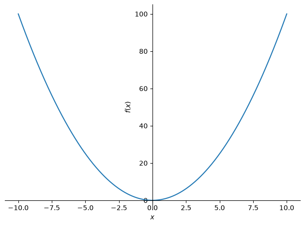
Note: the last line points to the result in the form of a Plot instance; we hide the output of the object <sympy.plotting.plot.Plot at 0x...> by using a semicolon:

plot(x**2);

but the figure is still displayed.

Some common arguments are:

• show displays the figure (default True),

• line_color the color of the plot,

• xscale and yscale the display mode (options: linear or log),

• xlim and ylim the display limits for the axes (a tuple of two (min, max) values).

Let’s prepare two figures where the $y$ axis is logarithmic and the plot range is from 1 to 5:

Now we extend the first figure with the second and display the result:

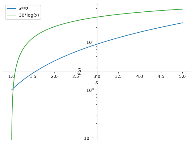
Parametric plot¶

Similarly, we use the function sympy.plotting.plot_parametric for a parametric plot (documentation):

plot_parametric(expr_x, expr_y, range, **kwargs)

where the new arguments are:

• expr_x and expr_y the definitions of the position of coordinates $x$ and $y$,

• **kwargs a dictionary of options.

We import the function:

Let’s show its use with an example:

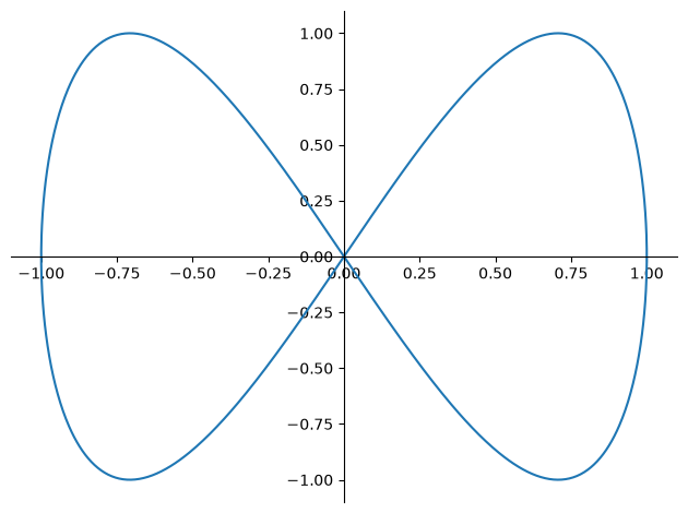
Plotting in space¶

The function sympy.plotting.plot3D (documentation) for plotting in space has the syntax:

plot3d(expression, range_x, range_y, **kwargs)

where the arguments are:

• expression the definition of the surface,

• range_x and range_y the range of coordinate x and y,

• **kwargs a dictionary of options.

We import the function:

Let’s show its use with an example:

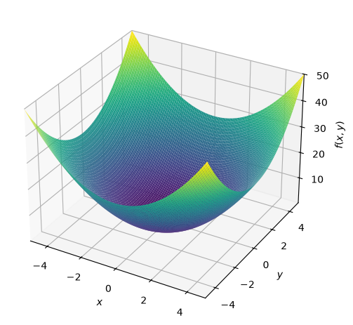
For other plots, see the documentation.

Algebra¶

In this section we will look at some of the basics of using SymPy for algebraic operations.

Using expand and factor¶

Let’s define a mathematical expression:

and now expand it (see the documentation):

If we want to look at the coefficients in front of x, we do it with the coeff() method:

The arguments of the function define what kind of expansion we want (documentation). If we want, e.g., a trigonometric expansion, then we use trig=True:

The inverse operation of expansion is factorization (documentation):

If we are interested in the individual factors, then we do this with the sympy.factor_list function:

Simplifying expressions with simplify¶

The sympy.simplify() function (documentation) tries to simplify expressions into simpler ones (e.g., by canceling variables).

For special purposes we can also simplify with:

• sympy.trigsimp,

• sympy.powsimp,

• sympy.logcombine.

For more, see the documentation.

Examples of simplification:

Using apart and together¶

We use these functions to work with fractions:

We perform partial fraction decomposition with the sympy.apart() function (documentation):

and then back again in the opposite direction with the sympy.together() function:

In the latter case we arrive at a similar result with sympy.simplify():

Differentiation¶

Differentiation is in principle a relatively simple mathematical operation, which we perform with the sympy.diff() function (documentation):

Let’s prepare an example:

Let’s differentiate it with respect to $x$:

or also

Higher-order derivatives are defined like this:

or (the same result a bit differently):

The derivative with respect to several variables $\frac{d^3f}{dx\,dy^2}$ is performed like this:

Integration¶

The integrate function can be used for indefinite integration (documentation):

integrate(f, x)

or for definite integration:

integrate(f, (x, a, b))

where the arguments are:

• f the function we integrate,

• x the variable with respect to which we integrate,

• a and b the limits of integration.

An example of indefinite integration:

We notice that sympy correctly takes into account the possibility that $y=0$.

Another example of definite integration:

An example where the limits are at infinity (we use the constant for infinity sympy.oo):

Sum and product of a series¶

We define the sum of a series with the sympy.Sum() function (documentation):

sympy.Sum(expression, (var, start, end))

where the arguments are:

• expression the expression we are summing,

• var, start and end the variable that increases from start to end (end is included).

An example of the sum of a series:

Only when we use the doit() method is the computation carried out:

Let’s also look at the numerical result:

We define the product of a series similarly with the sympy.Product function (documentation):

sympy.Product(expression, (var, start, end))

where the arguments are:

• expression the expression we are multiplying,

• var, start and end the variable that increases from start to end (end is included).

Example:

Limits¶

We compute limits with the sympy.limit() function (documentation):

sympy.limit(f, x, x0)

where the arguments are:

• f the expression whose limit we are seeking,

• x the variable that approaches x0,

• x0 the limit point.

Example:

As an example, let’s look at the use of the limit in the definition of the derivative:

Let’s prepare the function f and its derivative:

The derivative of the function is:

We compute the same result also using the limit:

Taylor series¶

We compute Taylor series with the sympy.series() function (documentation):

sympy.series(expression, x=None, x0=0, n=6, dir='+')

where the arguments are:

• expression the expression whose series we are determining,

• x the independent variable,

• x0 the value around which we determine the series (default 0),

• n the order of the series (default 6),

• dir the direction of the series expansion (+ or -).

Example:

If we want to define a different expansion point (x0=2) and use more terms (n=8), we do it like this:

The result also includes the order of validity; in this way we can control the validity of the computation ($\mathcal{O}$).

Example:

The computations s1 and s2 have different orders of validity, so the product:

is accurate only up to order $\mathcal{O}(x^2)$, which sympy handles appropriately:

The information about the order of validity can be removed:

Linear algebra¶

Matrices and vectors¶

We define matrices and vectors with the Matrix function. While with numpy.array it is not necessary to strictly adhere to the mathematical notation of vectors and matrices, with sympy it is required.

Let’s look at an example; first we prepare the variables:

Then the matrix and the column vector:

Now let’s look at some typical operations; first the multiplication of a matrix and a vector:

Then the dot product of two vectors (we must be careful to transpose one of the vectors):

The determinant and the inverse matrix:

Multiplication and power of a matrix:

Root finding (solving equations)¶

We solve equations and systems of equations with the sympy.solve() function (documentation). Solving the following equations is supported:

• polynomial equations,

• transcendental equations,

• piecewise-defined equations as a combination of the above two types,

• systems of linear and polynomial equations,

• systems of equations with inequalities.

The syntax is:

sympy.solve(f, *symbols, **flags)

where the arguments are:

• f an expression or a list of expressions,

• *symbols the symbol or list of symbols we want to determine,

• **flags a dictionary of options.

Let’s look at an example:

Let’s plot the solution (notice that we found only two of the infinitely many solutions):

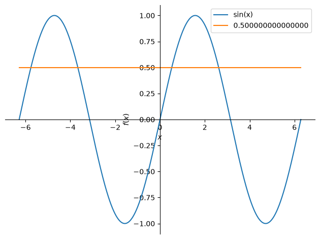
A quadratic equation:

A system of equations:

For nonlinear systems we can also use numerical solving with the sympy.nsolve() function (documentation):

sympy.nsolve(f, [args,] x0, modules=['mpmath'], **kwargs)

where the arguments are:

• f the equation or system of equations we are solving,

• args the variables (optional),

• x0 the initial estimate (a scalar or a vector),

• modules the package used to compute the numerical value (the same logic as with the lambdify function; the default is the mpmath package),

• **kwargs a dictionary of options.

Let’s look at the example from above:

Solving differential equations¶

Undefined functions¶

Before we look at differential equations, we must get to know undefined functions. We define such functions with sympy.Function documentation.

As an example, let’s look at how we define the equation $\ddot x(t)=g$. First let’s define the undefined function:

Then the symbols:

And the equation:

Differential equations¶

We solve differential equations and systems of differential equations with the sympy.dsolve() function (documentation):

sympy.dsolve(eq, func=None, hint='default', simplify=True,
             ics=None, xi=None, eta=None, x0=0, n=6, **kwargs)

where the selected arguments are:

• eq the differential equation or system of differential equations,

• func the solution we are seeking,

• ics the initial and boundary conditions of the differential equation.

Let’s look at the example of a mass $m$ sliding on a surface with friction coefficient $\mu$; the initial velocity is $v_0$, and the displacement $x_0=0$.

Let’s define the symbols:

Let’s define the differential equation:

Let’s look at the properties of the differential equation:

Let’s solve it:

We retrieve the right-hand side of the equation like this (rhs - right-hand side):

Additional¶

sympy.mechanics¶

sympy has built-in support for classical mechanics (documentation). A comprehensive tutorial was presented at the scientific conference SciPy 2016.