Numerical integration

Introduction¶

In this chapter, for a given function $f(x)$ we will compute the definite integral:

\int_a^b\,f(x)\,\textrm{d}x

(1)

where $a$ and $b$ are the limits of integration, and $f(x)$ are the function values obtained either from a table of values or from an analytical function.

In numerical integration, the integral is estimated by $I$ , and the following holds:

\int_a^b\,f(x)\,\textrm{d}x= I + E,

(2)

where $E$ is the error of the integral estimate.

We will compute the numerical integral based on a discrete sum:

I=\sum_{i=0}^{m}A_i\,f(x_i),

(3)

where $A_i$ are the weights, $x_i$ are the nodes on the interval $[a, b]$ , and $m+1$ is the number of nodes.

We will look at two different approaches to numerical integration:

the Newton-Cotes approach, which is based on equidistant nodes (a constant integration step), and
the Gaussian integration approach, where the nodes are placed so as to achieve exactness for polynomials.

Motivational example¶

For numerical integration, we will use a concrete example to guide us:

\int_1^2 x\,\sin(x)\,\textrm{d}x

(4)

Let us prepare the nodes. Let the basic step be $h=0.25$ ; in this case we have four subintervals and five nodes, at step $2h$ there are three nodes, and at step $4h$ only two (the endpoints):

import numpy as np
xg, hg = np.linspace(1, 2, 100, retstep=True) # dense points (for plotting)
x2v, h2v = np.linspace(1, 2, 2, retstep=True)  # step h2v = 1 (2 nodes)
x3v, h3v = np.linspace(1, 2, 3, retstep=True)  # step h3v = 0.5 (3 nodes)
x4v, h4v = np.linspace(1, 2, 4, retstep=True)  # step h4v = 0.33.. (4 nodes)
x5v, h5v = np.linspace(1, 2, 5, retstep=True)  # step h5v = 0.25 (5 nodes)

Let us also prepare the function values:

yg = xg * np.sin(xg)
y2v = x2v * np.sin(x2v)
y3v = x3v * np.sin(x3v)
y4v = x4v * np.sin(x4v)
y5v = x5v * np.sin(x5v)

Let us prepare a plot of the data:

import matplotlib.pyplot as plt
%matplotlib inline
def fig_motivation():
    plt.fill_between(xg, yg, alpha=0.25, facecolor='r')
    plt.annotate(r'$\int_1^2\,x\,\sin(x)\,\mathrm{d}x$', (1.3, 0.5), fontsize=22)
    plt.plot(xg, yg, lw=3, alpha=0.5, label=r'$x\,\sin(x)$')
    plt.plot(x2v, y2v, 's', alpha=0.5, label=f'$h={h2v}$', markersize=14)
    plt.plot(x3v, y3v, 'o', alpha=0.5, label=f'$h={h3v}$', markersize=10)
    plt.legend(loc=(1.01, 0))
    plt.ylim(0, 2)
    plt.show()

Let us display the data:

fig_motivation()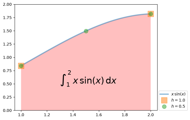

Let us compute the exact result analytically:

import sympy as sym
sym.init_printing()
x = sym.symbols('x')
I_exact = float(sym.integrate(x*sym.sin(x), (x, 1, 2)).evalf())
I_exact

Loading...

Newton-Cotes approach¶

The figure shows a general case in which the distance between the nodes $x_i$ is equal to $h$ (this is an equidistant partition). Integration

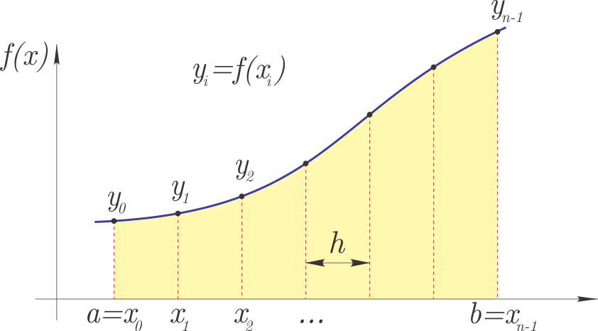
In this chapter we will first look at the trapezoidal and the composite trapezoidal rule, and later the Simpson’s and Romberg methods will follow.

Trapezoidal rule¶

The trapezoidal rule interpolates the values of the integrand $f(x)$ on the (sub)interval $[x_0, x_1]$ with a linear function. For two nodes, this means that we approximate the area under the graph of the function as:

I_{\textrm{trapezno}}=\sum_{i=0}^{1}A_i\,f(x_i)=\frac{h}{2}\cdot\left(f(x_0)+f(x_1)\right).

(5)

And the weights are:

A_0 = A_1 = \frac{1}{2}\,h.

(6)

Numerical implementation¶

The numerical implementation is:

def trapezoidal(y, h):
    """
    Trapezoidal rule of integration.

    :param y: function values
    :param h: integration step
    """
    return (y[0] + y[-1])*h/2

Numerical example¶

In our concrete case this means that we weight the first and last function value by $h/2$ . In our example $h=1$ :

I_trapezoidal = trapezoidal(y2v, h=h2v)
I_trapezoidal

Loading...

Let us prepare a figure:

def fig_trapezoidal():
    plt.fill_between(x2v, y2v, alpha=0.25, facecolor='r')
    plt.vlines(x2v, 0, y2v, color='r', linestyles='dashed', lw=1)
    plt.annotate('$I_{\\mathrm{trapezno}}$', (1.4, 0.5), fontsize=22)
    plt.annotate('Error', fontsize=20, xy=(1.5, 1.4), xytext=(1.6, 1.8),
            arrowprops=dict(facecolor='gray', shrink=0.05))
    plt.plot(xg, yg, lw=3, alpha=0.5, label='$x\\,\\sin(x)$')
    plt.plot(x2v, y2v, 'o', alpha=0.5, label=f'$h={h2v}$')
    plt.legend(loc=(1.01, 0))
    plt.ylim(0, 2)
    plt.show()

We display:

fig_trapezoidal()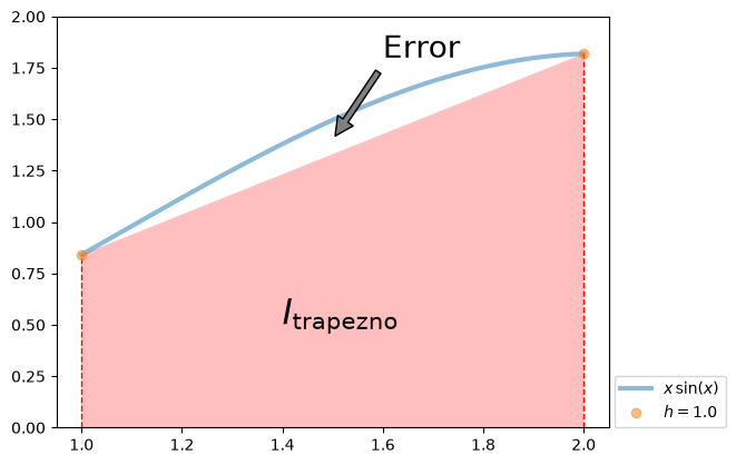

Error of the trapezoidal rule¶

The difference between the analytical value of the integral and the numerical approximation $I$ is the error of the method:

E = \int_a^bf(x)\,d x-I,

(7)

If the function $f(x)$ is at least twice differentiable, one can derive (see, e.g., the reference: Burden, Faires, Burden: Numerical Analysis 10th Ed) an error estimate that applies only to the trapezoidal approximation over the entire integration interval:

E_{\textrm{trapezno}}=-\frac{h^3}{12}f''(\xi),

(8)

where $h=b-a$ and $\xi$ is an unknown value on the interval $[a,b]$ .

Composite trapezoidal rule¶

If we divide the interval $[a, b]$ into $n$ subintervals and apply the trapezoidal rule of integration on each of them, we speak of the composite trapezoidal rule.

In this case, for each subinterval $i$ we apply the trapezoidal rule, and thus for the bounds of the subinterval $x_i$ and $x_{i+1}$ we use the weights $A_i=A_{i+1}=h/2$ . Since the interior nodes are doubled, it follows that:

A_0=A_{n}=\frac{h}{2}\quad\textrm{and for the other nodes:}\quad A_i=h.

(9)

Here we have assumed subintervals of equal width:

h=\frac{x_{n}-x_0}{n}

(10)

It therefore follows that:

I_{\textrm{trapezno sest}}=\sum_{i=0}^{n}A_i\,f(x_i)=\left(\frac{y_0}{2} + y_1+y_2+\cdots+y_{n-1}+\frac{y_{n}}{2}\right)\,h.

(11)

Numerical implementation¶

The numerical implementation is:

def trapezoidal_comp(y, h):
    """
    Composite trapezoidal rule of integration.

    :param y: function values
    :param h: integration step
    """
    return (np.sum(y) - 0.5*y[0] - 0.5*y[-1])*h

Numerical example¶

Above we already prepared the data for two subintervals (three nodes):

x3v

array([1. , 1.5, 2. ])

h3v

Loading...

Let us compute the estimate of the integral with the composite trapezoidal rule:

I_trapezoidal_comp = trapezoidal_comp(y3v, h=h3v)
I_trapezoidal_comp

Loading...

Let us prepare a figure:

def fig_trapezoidal_comp():
    plt.fill_between(x3v, y3v, alpha=0.25, facecolor='r')
    plt.vlines(x3v, 0, y3v, color='r', linestyles='dashed', lw=1)
    plt.annotate('$I_{\\mathrm{trapezno\\;sestavljeno}}$', (1.2, 0.5), fontsize=22)
    plt.annotate('Error', fontsize=20, xy=(1.75, 1.68), xytext=(1.4, 1.8),
            arrowprops=dict(facecolor='gray', shrink=0.05))
    plt.annotate('Error', fontsize=20, xy=(1.2, 1.1), xytext=(1., 1.4),
            arrowprops=dict(facecolor='gray', shrink=0.05))
    plt.plot(xg, yg, lw=3, alpha=0.5, label='$x\\,\\sin(x)$')
    plt.plot(x3v, y3v, 'o', alpha=0.5, label=f'$h={h3v}$')
    plt.legend(loc=(1.01, 0))
    plt.ylim(0, 2)
    plt.show()

We display:

fig_trapezoidal_comp()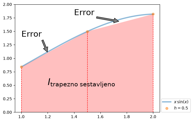

Error of the composite trapezoidal rule¶

The error of the composite trapezoidal rule stems from the error of the trapezoidal rule; here we make such an error $n$ times.

Since $h\cdot n=b-a$ holds, we derive the error of the composite trapezoidal rule as:

E_{\textrm{trapezno sest}}=-\frac{h^2(b-a)}{12}f''(\eta),

(12)

$\eta$ is a value on the interval $[a,b]$ . The error is of second order $\mathcal{O}(h^2)$ .

A better approximation of the integral¶

Next we will look at the so-called Richardson extrapolation, in which we compute a better approximation from the integral estimates with step $h$ and $2h$ .

If we compute the integral $I$ numerically at two different steps $h$ and $2\,h$ , the following holds:

\int_a^b f(x)\,\textrm{d}x = I_h + E_h = I_{2h} + E_{2h},

(13)

where $I_h$ and $I_{2h}$ are the approximations of the integral with step $h$ and $2h$ , and $E_h$ and $E_{2h}$ are the error estimates at step $h$ and $2h$ . We derive $I_{2h}-I_{h} = E_{h}-E_{2h}$

Next we write:

E_h=-\frac{h^2(b-a)}{12}f''(\eta)=h^2\,K.

(14)

Under the assumption that $f''\left (\eta \right )$ is the same at step $h$ and $2h$ ( $\eta$ is actually different at step $h$ and $2h$ ), we write:

E_{2h}=-\frac{(2h)^2(b-a)}{12}f''(\eta)=4\,h^2\,K

(15)

It follows that:

I_{2h}-I_h=-3K\,h^2.

(16)

Now we can estimate the error at step $h$ :

E_h=h^2\,K=\frac{I_h-I_{2h}}{3}.

(17)

Based on the error estimate, we can compute a better numerical approximation $I_{h}^*$ :

I_h^* = I_h + \frac{1}{3}\,(I_{h}-I_{2h})

(18)

or

I_h^* = \frac{4}{3}\,I_h - \frac{1}{3}\,I_{2h}

(19)

Numerical example¶

We previously computed the integral with the trapezoidal rule at step $h=1$ and at step $h=0.5$ already; the results were:

[I_trapezoidal, I_trapezoidal_comp]

Loading...

Using the formula above, we compute a better approximation:

I_trapezoidal_better = 4/3*I_trapezoidal_comp - 1/3*I_trapezoidal
print(f'Exact result:        {I_exact}\nBetter approximation: {I_trapezoidal_better}')

Exact result:        1.4404224209802097
Better approximation: 1.4408392930139313

The composite trapezoidal rule is also implemented in the numpy package, via the numpy.trapezoid function (numpy.trapz in older versions):

trapezoid(y, x=None, dx=1.0, axis=-1)

y represents the table of function values,
x is an optional parameter and defines the nodes; if the parameter is not defined, equidistant nodes spaced by dx are assumed,
dx defines the (constant) integration step, with a default value of 1,
axis defines the axis along which to integrate (in case y is a multidimensional numeric array).

The function returns the computed integral according to the composite trapezoidal rule. More information can be found in the documentation.

`numpy` implementation of the composite trapezoidal rule¶

Let us look at an example:

#%%timeit
I_trapezoidal_np = np.trapezoid(y3v, dx=h3v)
I_trapezoidal_np

Loading...

Simpson’s and other methods¶

Above we looked at the trapezoidal rule, which is based on a linear interpolating function on an individual subinterval. With higher-order interpolation we can derive further integration methods.

We need to compute:

\int_{a}^b f(x)\,dx.

(20)

We tabulate the integrand $f(x)$ and interpolate the table with the Lagrange interpolating polynomial $P_n(x)$ of degree $n$ :

P_n(x)=\sum_{i=0}^{n}\,f(x_i)\,l_i(x),

(21)

where $y_i=f(x_i)$ are the function values at the nodes $x_i$ and the Lagrange polynomial $l_i$ is defined as:

l_i(x)=\prod_{j=0, j\ne i}^n \frac{x-x_j}{x_i-x_j}.

(22)

For the numerical computation of the integral $\int_{a}^b f(x)\,dx$ (the limits are: $a=x_0$ , $b=x_n$ ), instead of the function $f(x)$ we substitute the interpolating polynomial $P_n(x)$ into the integral:

I=\int_{x_0}^{x_{n}} P_n(x)\,dx=\int_{x_0}^{x_{n}} \sum_{i=0}^{n}\,f(x_i)\,l_i(x)\,dx.

(23)

Since integration is a linear operation, we can swap the integration and the sum:

I=\sum_{i=0}^{n}\,f(x_i)\,\underbrace{\int_{x_0}^{x_{n}} l_i(x)\,dx}_{A_i}.

(24)

We integrate the Lagrange polynomial and obtain the weights $A_i$ :

A_i = \int_{x_0}^{x_{n}} l_i(x)\,dx

(25)

Derivation of the trapezoidal rule using Lagrange polynomials¶

Let us look at how we can computationally derive the weights $A_i$ for the case of the trapezoidal rule using a first-degree Lagrange interpolating polynomial.

First, let us define the variable x, the nodes x0 and x1, and the step h in symbolic form:

x, x0, x1, h = sym.symbols('x x0, x1, h')

Let us prepare a Python function that returns, in symbolic form, a list of $n$ coefficients of the Lagrange polynomials $[l_0(x), l_1(x),\dots, l_{n-1}(x)]$ of degree $n-1$ :

def lagrange(n, x, nodes_prefix='x'):
    if isinstance(nodes_prefix, str):
        nodes = sym.symbols(f'{nodes_prefix}:{n}')
    coeffs = []
    for i in range(0, n):
        numer = []
        denom = []

        for j in range(0, n):
            if i == j:
                continue

            numer.append(x    - nodes[j])
            denom.append(nodes[i] - nodes[j])

        numer = sym.Mul(*numer)
        denom = sym.Mul(*denom)

        coeffs.append(numer/denom)
    return coeffs

First, let us look at the Lagrange polynomials for linear interpolation ( $n=2$ ):

lag = lagrange(2, x)
lag

Loading...

Now we integrate the Lagrange polynomial $l_0(x)$ over the entire interval:

int0 = sym.integrate(lag[0], (x, x0, x1))
int0

Loading...

We simplify the expression and obtain:

int1 = int0.factor()
int1

Loading...

Since the width of the subinterval is constant, $x_1=h_0+h$ , we perform the substitution:

substitutions = {x1: x0+h}
int1.subs(substitutions)

Loading...

The steps above for the Lagrange polynomial $l_0(x)$ can be generalized to a list of Lagrange polynomials:

x, x0, x1, h = sym.symbols('x, x0, x1, h')
substitutions = {x1: x0+h}
A_trapezoid = [sym.integrate(li, (x, x0, x1)).factor().subs(substitutions)
            for li in lagrange(2, x)]  # for each Lagrange polynomial `li` in the list lagrange(2,x)
A_trapezoid

Loading...

We derived the weights that we used in the trapezoidal method:

A_0=h/2\qquad A_1=h/2.

(26)

The trapezoidal rule is:

I_{\textrm{trapezno}}=\frac{h}{2}\left(y_0+y_1\right)

(27)

The error estimate is (reference: Burden, Faires, Burden: Numerical Analysis 10th Ed):

E_{\textrm{trapezno}}= -\frac{h^3}{12}f''(\xi).

(28)

Computing the weights for Simpson’s rule¶

After showing the concise computation for the trapezoidal rule above, we can proceed similarly for quadratic interpolation over three points ( $n=3$ ).

The computation of the weights is analogous to the one above:

x, x0, x1, x2, h = sym.symbols('x, x0, x1, x2, h')
substitutions = {x1: x0+h, x2: x0+2*h}
A_Simpson1_3 = [sym.integrate(li, (x, x0, x2)).factor().subs(substitutions).factor()
             for li in lagrange(3, x)]
A_Simpson1_3

Loading...

Simpson’s rule (this rule is also called Simpson’s 1/3 rule) is:

I_{\textrm{Simpsonovo}}=\frac{h}{3}\left(y_0+4\,y_1+y_2\right)

(29)

The error estimate is (reference: Burden, Faires, Burden: Numerical Analysis 10th Ed):

E_{\textrm{Simpsonovo}}= -\frac{h^5}{90}f^{(4)}(\xi).

(30)

It should be pointed out that the error is locally of fifth order $\mathcal{O}(h^5)$ and is defined by the unknown value of the fourth derivative $f^{(4)}(\xi)$ ; consequently, this rule is exact for polynomials of degree 3 or less.

Example of use:

I_Simps = h3v/3 * np.sum(y3v * [1, 4, 1])
I_Simps

Loading...

Let us prepare a figure. Since Simpson’s rule is based on quadratic interpolation, we must first prepare the interpolating polynomial (we use scipy.interpolate):

from numpy.polynomial import Polynomial # interpolating polynomial through the nodes

def fig_simpson():
    y_interpolate = Polynomial.fit(x3v, y3v, deg=len(x3v)-1)
    plt.fill_between(xg, y_interpolate(xg), alpha=0.25, facecolor='r')
    plt.vlines(x3v, 0, y3v, color='r', linestyles='dashed', lw=1)
    plt.annotate('$I_{\\mathrm{Simpsonovo}}$', (1.2, 0.5), fontsize=22)
    plt.annotate('Error', fontsize=20, xy=(1.75, 1.7), xytext=(1.4, 1.8),
            arrowprops=dict(facecolor='gray', shrink=0.05))
    plt.annotate('Error', fontsize=20, xy=(1.2, 1.1), xytext=(1., 1.4),
            arrowprops=dict(facecolor='gray', shrink=0.05))
    plt.plot(xg, yg, lw=3, alpha=0.5, label='$x\\,\\sin(x)$')
    plt.plot(x3v, y3v, 'o', alpha=0.5, label=f'$h={h3v}$')
    plt.legend(loc=(1.01, 0))
    plt.ylim(0, 2)
    plt.show()

We display:

fig_simpson()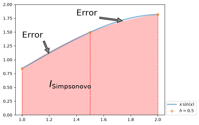

`scipy.integrate.newton_cotes`¶

The coefficients of the Newton-Cotes integration approach can also be obtained using scipy.integrate.newton_cotes() (documentation):

newton_cotes(rn, equal=0)

where the parameters are:

rn, which defines the number of subintervals (a non-constant step is also possible, see the documentation),
equal, which defines whether equally wide subintervals are required.

The function returns a tuple, in which the first element represents the numeric array of weights and the second element the error estimate.

Let us look at an example:

from scipy import integrate
integrate.newton_cotes(2)

(array([0.33333333, 1.33333333, 0.33333333]), -0.011111111111111112)

Computing the weights for Simpson’s 3/8 rule¶

We can continue with cubic interpolation over four points ( $n=4$ ):

x, x0, x1, x2, x3, h = sym.symbols('x, x0, x1, x2, x3, h')
substitutions = {x1: x0+h, x2: x0+2*h, x3: x0+3*h}
A_Simpson3_8 = [sym.integrate(li, (x, x0, x3)).factor().subs(substitutions).factor()
                for li in lagrange(4, x)]
A_Simpson3_8

Loading...

Simpson’s 3/8 rule is:

I_{\textrm{Simpsonovo 3/8}}=\frac{3h}{8}\left(y_0+3\,y_1+3\,y_2+y_3\right)

(31)

The error estimate is (reference: Burden, Faires, Burden: Numerical Analysis 10th Ed):

E_{\textrm{Simpsonovo 3/8}}= -\frac{3\,h^5}{80}f^{(4)}(\xi).

(32)

Let us look at an example of use. We use the previously prepared table of function values at four points:

y4v

array([0.84147098, 1.2959172 , 1.65901326, 1.81859485])

I_Simps38 = 3*h4v/8 * np.sum(y4v * [1, 3, 3, 1])
I_Simps38

Loading...

Let us also prepare a plot:

def fig_simpson38():
    y_interpolate = Polynomial.fit(x4v, y4v, deg=len(x4v)-1)
    plt.fill_between(xg, y_interpolate(xg), alpha=0.25, facecolor='r')
    plt.vlines(x4v, 0, y4v, color='r', linestyles='dashed', lw=1)
    plt.annotate('$I_{\\mathrm{Simpsonovo\\;3/8}}$', (1.2, 0.5), fontsize=22)
    plt.annotate('Error', fontsize=20, xy=(1.75, 1.7), xytext=(1.4, 1.8),
            arrowprops=dict(facecolor='gray', shrink=0.05))
    plt.annotate('Error', fontsize=20, xy=(1.5, 1.47), xytext=(1.1, 1.6),
            arrowprops=dict(facecolor='gray', shrink=0.05))
    plt.annotate('Error', fontsize=20, xy=(1.2, 1.1), xytext=(1., 1.4),
            arrowprops=dict(facecolor='gray', shrink=0.05))
    plt.plot(xg, yg, lw=3, alpha=0.5, label='$x\\,\\sin(x)$')
    plt.plot(x4v, y4v, 'o', alpha=0.5, label=f'$h={h4v:.6f}$')
    plt.legend(loc=(1.01, 0))
    plt.ylim(0, 2)
    plt.show()

We display:

fig_simpson38()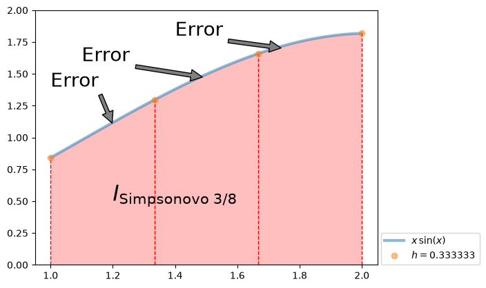

Composite Simpson’s rule¶

We divide the interval $[a, b]$ into an even number $n$ of subintervals of equal width $h=(b - a)/n$ , which defines the nodes $x_i=a+i\,h$ for $i=0,1,\dots,n$ . In this case we write the composite Simpson’s rule:

\int_{a}^{b}f(x)\,\textrm{d}x= \frac{h}{3}\left( f(x_0) +4\sum_{i=1}^{n/2}f(x_{2i-1}) +2\sum_{i=1}^{n/2-1}f(x_{2i}) +f(x_n) \right) \underbrace{ -\frac{b-a}{180}h^4\,f^{(4)}(\eta) }_{E_{\textrm{Sestavljeno Simpsonovo 1/3}}} ,

(33)

where $\eta$ is an unknown value on the interval $[a, b]$ . The error is of fourth order $\mathcal{O}(h^4)$ .

Numerical implementation:

def simpson_comp(y, h):
    """
    Composite Simpson's rule of integration.

    :param y: function values
    :param h: integration step
    """
    return h/3 * (y[0] + 4*np.sum(y[1:-1:2]) + 2*np.sum(y[2:-1:2]) + y[-1])

I_Simps_comp = simpson_comp(y5v, h=h5v)
I_Simps_comp

Loading...

Let us prepare a figure:

def fig_simpson_comp():
    y_interpolate = Polynomial.fit(x5v, y5v, deg=len(x5v)-1)
    plt.fill_between(xg, y_interpolate(xg), alpha=0.25, facecolor='r')
    plt.vlines(x5v, 0, y5v, color='r', linestyles='dashed', lw=1)
    plt.annotate('$I_{\\mathrm{Simpsonovo\\;sestavljeno}}$', (1.2, 0.5), fontsize=22)
    plt.annotate('Error', fontsize=20, xy=(1.70, 1.68), xytext=(1.4, 1.8),
            arrowprops=dict(facecolor='gray', shrink=0.05))
    plt.plot(xg, yg, lw=3, alpha=0.5, label='$x\\,\\sin(x)$')
    plt.plot(x5v, y5v, 'o', alpha=0.5, label=f'$h={h5v}$')
    plt.legend(loc=(1.01, 0))
    plt.ylim(0, 2)
    plt.show()

We display:

fig_simpson_comp()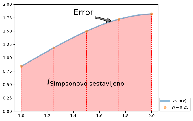

A better estimate of the integral¶

The error of the composite Simpson’s method is defined by:

E_{\textrm{Sestavljeno Simpsonovo 1/3}}= -\frac{b-a}{180}h^4\,f^{(4)}(\eta),

(34)

where $\eta$ is an unknown value on the interval $[a, b]$ .

We determine an improved estimate of the integral in a manner similar to the composite trapezoidal method; we estimate the integral $I$ at two different steps $h$ and $2\,h$ , and the following holds exactly:

\int_a^b f(x)\,\textrm{d}x = I_h + E_h = I_{2h} + E_{2h},

(35)

where $I_h$ is the approximation of the integral with step $h$ and $E_h$ is the error estimate at step $h$ ; the same holds analogously for $I_{2h}$ and $E_{2h}$ .

If we assume that $f^{(4)}\left (\eta \right )$ is the same in both cases, we can determine the difference $I_{2h}-I_{h} = E_{h}-E_{2h}$ .

Next we write:

E_h=-\frac{b-a}{180}h^4\,f^{(4)}(\eta)=h^4\,K.

(36)

Under the assumption that $f^{(4)}\left (\eta \right )$ is the same at step $h$ and $2h$ ( $\eta$ is actually different at step $h$ and $2h$ ), we write:

E_{2h}=-\frac{(b-a)}{180}(2h)^4\,f^{(4)}(\eta)=16\,h^4\,K

(37)

It follows that:

I_{2h}-I_h=-15K\,h^4.

(38)

Now we can estimate the error at step $h$ :

E_h=h^4\,K=\frac{I_h-I_{2h}}{15}.

(39)

Based on the error estimate, we can compute a better approximation $I_{h}^*$ :

I_h^* = I_h + \frac{1}{15}\,(I_{h}-I_{2h})

(40)

or

I_h^* = \frac{16}{15}\,I_h - \frac{1}{15}\,I_{2h}

(41)

Numerical example¶

We previously computed the integral with Simpson’s rule at step $h=0.5$ and at step $h=0.25$ already; the results were:

[I_Simps, I_Simps_comp]

Loading...

Using the formula above, we compute a better approximation:

I_Simps_better = 16/15*I_Simps_comp - 1/15*I_Simps
print(f'Exact result:        {I_exact}\nBetter approximation: {I_Simps_better}')

Exact result:        1.4404224209802097
Better approximation: 1.4404218714139077

We obtain a better numerical approximation, but we lose the error estimate!

Simpson’s method in `scipy.integrate.simpson`¶

The composite Simpson’s rule is implemented in scipy in scipy.integrate.simpson() (documentation):

simpson(y, x=None, *, dx=1.0, axis=-1)

where the parameters are:

y the table of function values that we integrate,
x the nodes, an optional parameter; if x=None, equidistant subintervals of width dx are assumed,
dx the width of the equidistant subintervals, i.e., the integration step,
axis the integration axis (important in the case of a multidimensional numeric array).

In older SciPy versions the function was called simps and also had the parameter even; both were removed in SciPy 1.14.

Let us look at an example; first we import the simpson function:

from scipy.integrate import simpson

#%%timeit
simpson(y5v, dx=h5v)

Loading...

Romberg method¶

The Romberg method is based on Richardson extrapolation. Let us assume that we integrate the integral $\int_a^b f(x)\textrm{d}x$ on the interval $[a,b]$ , which we divide into $2^{n-1}$ subintervals ( $n=1,2,4,8, \dots$ ).

We denote the result of the trapezoidal rule at $n=1$ by $R_{\underbrace{1}_{n},\underbrace{1}_{j}}$ , where $j$ denotes the accuracy of the obtained result $\mathcal{O}(h^{2j})$ .

If we apply the trapezoidal integration rule at $n=1,2,4 \dots$ subintervals, we compute:

$R_{1,1}$ , step $h_1=h$ , order of accuracy $\mathcal{O}(h_1^2)$ ,
$R_{2,1}$ , step $h_2=h/2$ , order of accuracy $\mathcal{O}(h_2^2)$ ,
$R_{3,1}$ , step $h_3=h/4$ , order of accuracy $\mathcal{O}(h_3^2)$ ,
$R_{4,1}$ , step $h_4=h/8$ , order of accuracy $\mathcal{O}(h_4^2)$ ,
$\dots$
$R_{n,1}$ , step $h_4=h/(2^{n-1})$ , order of accuracy $\mathcal{O}(h_n^2)$ .

Based on Richardson extrapolation we compute a better approximation

$R_{2,2} = R_{2,1} + \frac{1}{3}\left(R_{2,1}-R_{1,1}\right)$ , step $h_2=h/2$ , order of accuracy $\mathcal{O}(h_2^4)$ ,
$R_{3,2} = R_{3,1} + \frac{1}{3}\left(R_{3,1}-R_{2,1}\right)$ , step $h_3=h/4$ , order of accuracy $\mathcal{O}(h_3^4)$ ,
$\dots$
$R_{n,2} = R_{n,1} + \frac{1}{3}\left(R_{n,1}-R_{n-1,1}\right)$ , step $h_n=h/(2^{n-1})$ , order of accuracy $\mathcal{O}(h_n^4)$ .

Then we continue with Richardson extrapolation:

$R_{3,3} = R_{3,2} + \frac{1}{15}\left(R_{3,2}-R_{2,2}\right)$ , step $h_3=h/4$ , order of accuracy $\mathcal{O}(h_3^6)$ ,
$\dots$
$R_{n,3} = R_{n,2} + \frac{1}{15}\left(R_{n,2}-R_{n-1,2}\right)$ , step $h_n=h/(2^{n-1})$ , order of accuracy $\mathcal{O}(h_n^6)$ .

Richardson extrapolation can be generalized:

$R_{n,j} = R_{n,j-1} + \frac{1}{4^{j-1}-1}\left(R_{n,j-1}-R_{n-1,j-1}\right)$ , step $h_n=h/(2^{n-1})$ , order of accuracy $\mathcal{O}(h_n^{2j})$

Here, the better approximation $R_{2,2}$ at step $h/2$ is equal to the result obtained by Simpson’s method at step $h/2$ . Similarly, the better approximation $R_{3,2}$ at step $h/4$ is equal to the numerical integral of Simpson’s method at step $h/4$ . And further, $R_{3,3}$ is equal to the corrected approximation of Simpson’s method at step $h/4$ .

Let us prepare the numerical data:

x9v, h9v = np.linspace(1, 2, 9, retstep=True)  # step h9v = 0.125 (9 nodes)
y9v = x9v * np.sin(x9v)

Let us look at the example from above. First, we compute the integral with the composite trapezoidal method at different steps (second-order error):

## O(h^2)
R1_1 = trapezoidal_comp(y9v[::8], 8*h9v) # h=1.0
R2_1 = trapezoidal_comp(y9v[::4], 4*h9v) # h=0.5
R3_1 = trapezoidal_comp(y9v[::2], 2*h9v) # h=0.25
R4_1 = trapezoidal_comp(y9v, h9v) # h=0.125
[R1_1, R2_1, R3_1, R4_1]

Loading...

Then we compute better approximations (we obtain a fourth-order error):

## O(h^4)
R2_2 = R2_1 + 1/3 * (R2_1 - R1_1)
R3_2 = R3_1 + 1/3 * (R3_1 - R2_1)
R4_2 = R4_1 + 1/3 * (R4_1 - R3_1)
[R2_2, R3_2, R4_2]

Loading...

The results represent the result of Simpson’s method at step $h=0.5$ , $h=0.25$ and $h=0.125$ :

[simpson_comp(y9v[::4], 4*h9v), simpson_comp(y9v[::2], 2*h9v), simpson_comp(y9v, h9v)]

Loading...

We again compute better approximations (we obtain a sixth-order error):

## O(h6)
R3_3 = R3_2 + 1/15 * (R3_2 - R2_2)
R4_3 = R4_2 + 1/15 * (R4_2 - R3_2)

[R3_3, R4_3]

Loading...

The result represents the better result of Simpson’s method at step $h=0.25$ and $h=0.125$ :

a4h, a2h, ah = [simpson_comp(y9v[::4], 4*h9v), simpson_comp(y9v[::2], 2*h9v), simpson_comp(y9v, h9v)]
[16/15*a2h-1/15*a4h, 16/15*ah-1/15*a2h]

Loading...

We again compute better approximations (we obtain an eighth-order error):

## O(h8)
R4_4 = R4_3 + 1/63 * (R4_3 - R3_3)
R4_4

Loading...

The Romberg method thus offers high result accuracy at a relatively low numerical cost. The error is estimated by:

E = \left|R_{n,n}-R_{n-1,n-1}\right|.

(42)

Romberg method in `scipy.integrate.romb`¶

The Romberg method is implemented in scipy in scipy.integrate.romb() (documentation):

romb(y, dx=1.0, axis=-1, show=False)

where the parameters are:

y the table of function values that we integrate,
dx the width of the equidistant subintervals, i.e., the integration step,
axis the integration axis (important in the case of a multidimensional numeric array),
show if True, displays the elements of the Richardson extrapolation.

Let us look at the example from above:

from scipy.integrate import romb

y9v

array([0.84147098, 1.01505104, 1.18623077, 1.34872795, 1.49624248,
       1.62261343, 1.72197541, 1.78891084, 1.81859485])

romb(y9v, dx=h9v, show=True)

Richardson Extrapolation Table for Romberg Integration
======================================================
 1.33003 
 1.41314  1.44084 
 1.43362  1.44045  1.44042 
 1.43872  1.44042  1.44042  1.44042 
======================================================

Loading...

Gaussian integration approach¶

The Newton-Cotes approach is based on a polynomial of degree $n$ , and the error is of degree $n+1$ . This means that the integration yields an exact result if the integrated function is a polynomial of degree $n$ or less; for even $n$ , owing to symmetry, even of degree $n+1$ (Simpson’s rule, $n=2$ , is e.g. exact also for cubic polynomials).

The Gaussian integration approach is fundamentally different: the goal is to replace the integral of the function $f(x)$ with a weighted sum of function values at discrete values $f(x_i)$ :

\int_a^bf(x)\,\textrm{d}x\approx \sum_{i=0}^{n-1} A_i\, f(x_i).

(43)

Here both the weight $A_i$ and the location of the node $x_i$ are unknown. For polynomials of degree $n$ we will also need more points $(x_i, f(x_i))$ .

In what follows, we will learn that we can compute a numerically exact integral very efficiently. An additional advantage of Gaussian integration is that it can compute the integral of functions with singularities (e.g.: $\int_0^1\sin(x)/\sqrt{(x)}\,dx$ ).

Gaussian quadrature with one node¶

Let us assume that we want to integrate a polynomial of degree $n=1$ (a linear function):

f(x)=P_1(x)=a_0+a_1\,x.

(44)

Let us compute:

\int_{x_L}^{x_D}P_1(x)\,\textrm{d}x=\left(a_0\,x+a_1\,\frac{x^2}{2}\right)_{x_L}^{x_D}=-a_0\,x_L+a_0\,x_D-\frac{a_1\,x_L^2}{2}+\frac{a_1\,x_D^2}{2}.

(45)

On the other hand, we want to compute the integral from the appropriately weighted $A_0$ value of the function $f(x_0)$ at an unknown node $x_0$ (only one node!):

\int_{x_L}^{x_D}P_1(x)\,\textrm{d}x = A_0\,P_1(x_0)= A_0\,a_0+A_0\,a_1\,x_0.

(46)

By equating the expressions above, we derive:

-a_0\,x_L+a_0\,x_D-\frac{a_1\,x_L^2}{2}+\frac{a_1\,x_D^2}{2}=A_0\,a_0+A_0\,a_1\,x_0.

(47)

$a_0$ and $a_1$ are the coefficients of the linear function, which can take arbitrary values, so it holds that:

a_0\,\left(-x_L+x_D-A_0\right)=0\qquad\textrm{and}\qquad a_1\left(-\frac{x_L^2}{2}+\frac{x_D^2}{2}-A_0\,x_0\right)=0.

(48)

This is a system of linear equations with the solution:

A_0= x_D-x_L, \qquad x_0=\frac{x_L+x_D}{2}.

(49)

If the integrated function is linear, we will compute the true value based only on the value at a single point!

So that the Gaussian integration approach is independent of the integration limits $x_L$ , $x_D$ , we introduce standard limits.

Standard limits: $x_L=-1$ and $x_D=1$ ¶

For generality, we transform the limits $x\in[x_L, x_D]$ into $\xi\in[-1, +1]$ using:

x=\frac{x_D+x_L}{2}+\frac{x_D-x_L}{2}\xi

(50)

and

\textrm{d}x=\frac{x_D-x_L}{2}\textrm{d}\xi.

(51)

The following holds:

\int_{x_L}^{x_D}f(x)\,\textrm{d}x=\int_{-1}^1 g\left(\xi\right)\,\textrm{d}\xi,

(52)

where:

g(\xi)=\frac{x_D-x_L}{2}\,f\left(\frac{x_L+x_D}{2}+\frac{x_D-x_L}{2}\xi\right).

(53)

In the case of standard limits, at one Gauss point the weight is $A_0=2$ and $x_0=0$ is the value at which we must evaluate the function $f(x_0)$ .

Computational derivation of the weights and the Gauss point¶

Let us define the symbols and set up the equation:

a_0, a_1, x, x_L, x_D, A_0, x_0 = sym.symbols('a_0, a_1, x, x_L, x_D, A_0, x_0') # symbols
P1 = a_0 + a_1*x                                                   # linear polynomial
eq = sym.Eq(P1.integrate((x, x_L, x_D)).expand(), A_0*P1.subs(x, x_0)) # theoretical integral = estimate with weights
eq

Loading...

Let us prepare two equations (for the first we assume $a_0=0, a_1=1$ , for the second we assume $a_0=1, a_1=0$ ) and solve the system for A_0 and x_0:

sym.solve([eq.subs(a_0, 0).subs(a_1, 1), eq.subs(a_1, 0).subs(a_0, 1)], [A_0, x_0])

Loading...

For additional explanation, I recommend this video.

Gaussian integration method with multiple nodes¶

We want to derive a Gaussian integration method that will take into account $v$ nodes on the interval $[a,b]$ and will exactly compute the integral of polynomials up to degree $n=2v-1$ . The following must hold:

\int_a^bP_{2v-1}(x)\,\textrm{d}x = \sum_{i=0}^{v-1} A_i\,P_{2v-1}(x_i).

(54)

In the derivation we will restrict ourselves to the standard limits $x_L=-1$ , $x_D=1$ ,

where the polynomial of degree $n=2v-1$ is defined as:

P_{2v-1}(x)=\sum_{i=0}^{2v-1} a_i\,x^i.

(55)

With two Gauss points/nodes we exactly compute the integral of a polynomial up to third order, and with three Gauss nodes we exactly compute the integral of a polynomial up to fifth order!

Computational derivation¶

Let us first prepare the symbolic notation of the polynomial and the corresponding variables:

def P_etc(n=1, a='a', x='x'):                       # n is the degree of the polynomial
    ai = sym.symbols(f'{a}:{n+1}')                  # list of a_i
    x = sym.symbols(x)                              # variable x
    return ai, x, sum([ai[i]*x**i for i in range(n+1)])

Now let us find the weights $A_i$ and the nodes $x_i$ for the case of two Gauss nodes; the polynomial is therefore of third degree.

v = 2 # number of nodes
ai, x, P = P_etc(n=2*v-1)
xi = sym.symbols(f'x:{v}') # list of x_i
Ai = sym.symbols(f'A:{v}') # list of A_i
print(f'Nodes:   {xi}\nWeights: {Ai}')

Nodes:   (x0, x1)
Weights: (A0, A1)

The polynomial:

Loading...

Similarly to the one node above, here let us define the equations:

eqs = [sym.Eq(P.integrate((x, -1, 1)).coeff(a_),\
              sum([Ai[i]*P.subs(x, xi[i]) \
                   for i in range(v)]).expand().coeff(a_)) \
       for a_ in ai]
eqs

Loading...

We solve them for the unknown $x_i$ and $A_i$ :

sol = sym.solve(eqs, sym.flatten((xi, Ai)))
sol

Loading...

We determined a list of two (equal) solutions.

First, the nodes are defined: $x_0=-\sqrt{3}/3$ and $x_1=\sqrt{3}/3$ , with the corresponding weights $A_0=A_1=1$ .

The code above is derived in general - you can increase the number of nodes v and compute the nodes and the corresponding weights.

Below is a table of nodes and weights for one, two, and three nodes (for the limits $a=-1$ , $b=1$ ):

Number of points 1:

$i$	Node $x_i$	Weight $A_i$
0	0	2

Number of points 2:

$i$	Node $x_i$	Weight $A_i$
0	$-\frac{\sqrt{3}}{3}$	1
1	$+\frac{\sqrt{3}}{3}$	1

Number of points 3:

$i$	Node $x_i$	Weight $A_i$
0	$-\frac{\sqrt{15}}{5}$	$\frac{5}{9}$
1	0	$\frac{8}{9}$
2	$\frac{\sqrt{15}}{5}$	$\frac{5}{9}$

For more nodes and also the error estimate, see Mathworld Legendre-Gauss Quadrature.

For the case of three Gauss points, we compute the numerical integral (standard limits):

I_{\textrm{Gauss3}}= \frac{5}{9}\,f\left(-\frac{\sqrt{15}}{5}\right) + \frac{8}{9}\,f\left(0\right)+\frac{5}{9}\,f\left(\frac{\sqrt{15}}{5}\right).

(56)

Numerical implementation¶

The numerical implementation (including the transformation of the limits) for one, two, or three nodes:

def gaussian(fun, a, b, nodes=1):
    """
    Gaussian integration method.

    :param fun: object of the function to integrate
    :param a:   lower limit
    :param b:   upper limit
    :param nodes: number of nodes (1, 2, or 3)
    """
    def g(xi): # function for transforming the limits
        return (b-a)/2 * fun((b+a +xi * (b-a))/2)

    if nodes == 1:
        return 2*g(0.)
    elif nodes == 2:
        return 1. * g(-np.sqrt(3)/3) + 1. * g(np.sqrt(3)/3)
    elif nodes == 3:
        return 5/9 * g(-np.sqrt(15)/5) +8/9 * g(0.) + 5/9 * g(np.sqrt(15)/5)

Let us look at an example. First, let us define the function we want to integrate:

def f(x):
    return x*np.sin(x)

Now we pass the function (in this concrete case f) and not the value (e.g., f(0.)) to the gaussian function. First for one node, then two and three:

gaussian(fun=f, a=1., b=2., nodes=1)

Loading...

gaussian(fun=f, a=1., b=2., nodes=2)

Loading...

gaussian(fun=f, a=1., b=2., nodes=3)

Loading...

`scipy.integrate.fixed_quad`¶

Within scipy, the Gaussian integration method is implemented in the scipy.integrate.fixed_quad() function (documentation):

fixed_quad(func, a, b, args=(), n=5)

where the parameters are:

func is the name of the function we call,
a is the lower limit,
b is the upper limit,
args is a tuple of any additional arguments of the function func,
n is the number of nodes of the Gaussian integration, default n=5.

The function returns a tuple with the integration result val and the value None: (val, None)

Let us look at the example from above:

from scipy.integrate import fixed_quad
fixed_quad(f, a=1, b=2, n=3)[0]

Loading...

The result is equal to the previous one:

gaussian(fun=f, a=1., b=2., nodes=3)

Loading...

`scipy.integrate`¶

scipy.integrate is a powerful tool for numerical integration (see the documentation). In what follows, we will look at some of the functions.

Integration functions that require a defining function:¶

quad(func, a, b[, args, full_output, ...]) computes the definite integral of func(x) over the limits [a, b],
dblquad(func, a, b, gfun, hfun[, args, ...]) computes the definite integral of func(x,y),
tplquad(func, a, b, gfun, hfun, qfun, rfun) computes the definite integral of func(x,y,z),
nquad(func, ranges[, args, opts, full_output]) computes the definite integral of the $n$ -dimensional function func( ...),

`scipy.integrate.quad`¶

Let us look at a very useful function for integration, scipy.integrate.quad() (documentation):

quad(func, a, b, args=(), full_output=0, epsabs=1.49e-08, epsrel=1.49e-08, limit=50,
     points=None, weight=None, wvar=None, wopts=None, maxp1=50, limlst=50)

The selected parameters are:

func the Python function we integrate,
a the lower limit of integration (np.inf can be used for an infinite limit),
b the upper limit of integration (np.inf can be used for an infinite limit),
full_output to display all results, default 0,
epsabs the allowed absolute error,
epsrel the allowed relative error.

Let us look at the example from above:

from scipy import integrate

integrate.quad(f, a=1, b=2)

Loading...

`scipy.integrate.dblquad`¶

This is a function similar to quad, but for integration over two variables (documentation). The function scipy.integrate.dblquad() computes the double integral of func(y, x) over the limits from x = [a, b] and y = [gfun(x), hfun(x)].

dblquad(func, a, b, gfun, hfun, args=(), epsabs=1.49e-08, epsrel=1.49e-08)

The selected parameters are:

func is the Python function we integrate,
a is the lower limit of integration of x (np.inf can be used for an infinite limit),
b is the upper limit of integration of x (np.inf can be used for an infinite limit),
gfun is the Python function that defines the lower limit of y as a function of x,
hfun is the Python function that defines the upper limit of y as a function of x.

Let us look at an example of computing the area of a half-circle with radius 1:

\int_{-1}^{1}\left(\int_0^{\sqrt{1-x^2}}1\,\textrm{d}y\right)\,\textrm{d}x=\frac{\pi}{2}

(57)

Let us define the appropriate Python functions and compute the result:

def func(y, x): # the integration function is simple, a constant = 1!
    return 1.
def gfun(x):    # lower limit = 0
    return 0.
def hfun(x):    # upper limit
    return np.sqrt(1-x**2)
integrate.dblquad(func=func, a=-1, b=1, gfun=gfun, hfun=hfun)

Loading...

Integration functions that require a table of values:¶

trapezoid(y[, x, dx, axis]) composite trapezoidal rule,
cumulative_trapezoid(y[, x, dx, axis, initial]) cumulative integral of the integrand (returns the result at each node),
simpson(y[, x, dx, axis]) Simpson’s method,
romb(y[, dx, axis, show]) Romberg method.

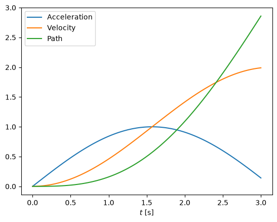
Here we will look at the cumulative_trapezoid function on an example. Consider the case where a mass $m=1$ (we omit the units) acted upon by a force $F=\sin(t)$ . From Newton’s 2nd law it follows that: $F=m\,\ddot x$ . We integrate the acceleration to compute the velocity; then we integrate once more for the displacement. Let us first define the function for the acceleration:

def acceleration(t):
    F = np.sin(t)
    m = 1
    return F/m

We are interested in what happens over a time of 3 seconds:

t, h = np.linspace(0, 3, 100, retstep=True)

Let us compute the table of accelerations and then integrate for the velocity (here it is important to define the initial value):

a = acceleration(t)
v = integrate.cumulative_trapezoid(y=a, dx=h, initial=0)

Now let us integrate the velocity once more to compute the path:

s = integrate.cumulative_trapezoid(y=v, dx=h, initial=0)

Let us display the result:

plt.plot(t, a, label='Acceleration')
plt.plot(t, v, label='Velocity')
plt.plot(t, s, label='Path')
plt.xlabel('$t$ [s]')
plt.legend();

Introduction¶

Motivational example¶

Newton-Cotes approach¶

Trapezoidal rule¶

Numerical implementation¶

Numerical example¶

Error of the trapezoidal rule¶

Composite trapezoidal rule¶

Numerical implementation¶

Numerical example¶

Error of the composite trapezoidal rule¶

A better approximation of the integral¶

Numerical example¶

numpy implementation of the composite trapezoidal rule¶

Simpson’s and other methods¶

Derivation of the trapezoidal rule using Lagrange polynomials¶

Computing the weights for Simpson’s rule¶

scipy.integrate.newton_cotes¶

Computing the weights for Simpson’s 3/8 rule¶

Composite Simpson’s rule¶

A better estimate of the integral¶

Numerical example¶

Simpson’s method in scipy.integrate.simpson¶

Romberg method¶

Romberg method in scipy.integrate.romb¶

Gaussian integration approach¶

Gaussian quadrature with one node¶

Standard limits: xL=−1x_L=-1xL​=−1 and xD=1x_D=1xD​=1¶

Computational derivation of the weights and the Gauss point¶

Gaussian integration method with multiple nodes¶

Computational derivation¶

Numerical implementation¶

scipy.integrate.fixed_quad¶

scipy.integrate¶

Integration functions that require a defining function:¶

scipy.integrate.quad¶

scipy.integrate.dblquad¶

Integration functions that require a table of values:¶

`numpy` implementation of the composite trapezoidal rule¶

`scipy.integrate.newton_cotes`¶

Simpson’s method in `scipy.integrate.simpson`¶

Romberg method in `scipy.integrate.romb`¶

Standard limits: $x_L=-1$ and $x_D=1$ ¶

`scipy.integrate.fixed_quad`¶

`scipy.integrate`¶

`scipy.integrate.quad`¶

`scipy.integrate.dblquad`¶