Approximation (curve fitting)

Introduction¶

In engineering practice we often encounter a table of data that may be affected by measurement or numerical errors.

Let us look at an example of measuring a (linear) spring ( $x$ is the displacement, $y$ is the measured force):

import numpy as np

x = np.array([0.1,  1.1, 2.05, 3.2, 3.9  ])
y = np.array([0.22, 18.15, 44.33, 75.59, 105.63])

Let us look at the data in a figure; first we import the required packages:

import matplotlib.pyplot as plt
%matplotlib inline
plt.plot(x, y, 'o');
plt.xlabel('Displacement $x$')
plt.ylabel('Force $y$');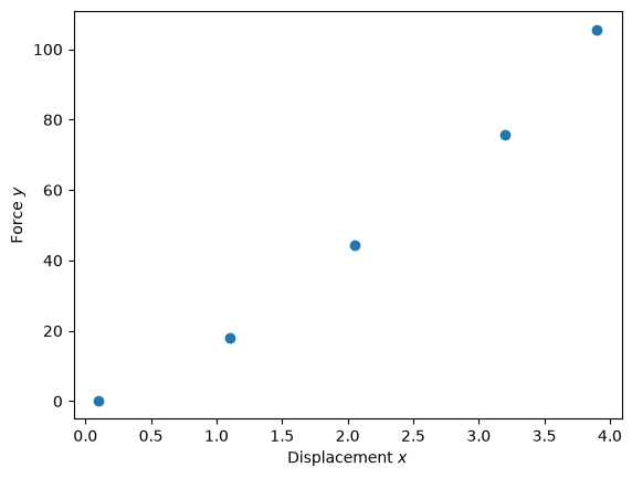

For this particular example, given our knowledge of the physical background of a linear spring, it would be appropriate to try to describe the measurements with a linear function:

f(x) = a_0\,x+ a_1

(1)

We know a table of $n$ data points $x_i, y_i$ for $i=0,1,\dots,n-1$ ; there are more of them than we need to determine the two constants $a_0$ and $a_1$ , so we have an overdetermined system of linear equations:

y_i=a_0\,x_i+a_1\quad\textrm{za}\quad i=0,1,\dots,n-1.

(2)

We are looking for values of the constants $a_0$ and $a_1$ such that the function $f(x)$ best matches $y_i$ at the known points $x_i$ .

So first we need a criterion for the best match.

For the values $x_i, y_i$ from the table we could look for values of $a_0$ and $a_1$ at which the sum of the absolute values of the deviations $P$ is the smallest:

P(a_0, a_1) = \sum_{i=0}^{n-1} |y_i - (a_0\,x_i+a_1)|.

(3)

However, since such a function $P(a_0, a_1)$ is not continuously differentiable, we prefer to use the least-squares method:

S(a_0, a_1) = \sum_{i=0}^{n-1} \left(y_i - (a_0\,x_i+a_1)\right)^2.

(4)

Such a function $S(a_0, a_1)$ is continuous and continuously differentiable. By taking partial derivatives with respect to the parameters $a_0$ and $a_1$ we can find a stationary point (the partial derivatives are equal to 0). We will go through the procedure for a linear function in the next section.

Least-squares method for a linear function¶

from IPython.display import YouTubeVideo
YouTubeVideo('8-oixY6GG9E', width=800, height=300)

Loading...

We need to find the constants $a_0$ , $a_1$ such that the sum of the squares of the differences between the function and the tabulated value ( $x_i, y_i$ , where $i=0,1,\dots, n-1$ and $n$ is the number of tabulated data points):

S(a_0, a_1) = \sum_{i=0}^{n-1} \left(y_i - (a_0\,x_i+a_1)\right)^2

(5)

is the smallest. The value will be smallest at the stationary point, which we determine by taking the partial derivative with respect to the parameters $a_0$ and $a_1$ .

First we take the partial derivative with respect to the parameter $a_0$ :

\frac{\partial S(a_0, a_1)}{\partial a_0} = 2\,\sum_{i=0}^{n-1} \left(y_i - a_0\,x_i-a_1\right)\,(-x_i)

(6)

We rearrange the expression:

\frac{\partial S(a_0, a_1)}{\partial a_0} =-2\left(\sum_{i=0}^{n-1} y_i\,x_i -a_0\,\sum_{i=0}^{n-1} x_i^2- a_1\,\sum_{i=0}^{n-1} x_i\right)

(7)

We proceed similarly for $a_1$ :

\frac{\partial S(a_0, a_1)}{\partial a_1} = 2\,\sum_{i=0}^{n-1} \left(y_i - a_0\,x_i- a_1\right)\,(-1)

(8)

\frac{\partial S(a_0, a_1)}{\partial a_1} = -2\left(\sum_{i=0}^{n-1} y_i -a_0\,\sum_{i=0}^{n-1} x_i- a_1\,\sum_{i=0}^{n-1}1\right)

(9)

Since at the stationary point $\partial S(a_0, a_1)/\partial a_0=0$ and $\partial S(a_0, a_1)/\partial a_1=0$ , from the expressions above we derive:

a_0\,\sum_{i=0}^{n-1} x_i^2 + a_1\,\sum_{i=0}^{n-1} x_i=\sum_{i=0}^{n-1} y_i\,x_i

(10)

and

a_0\,\sum_{i=0}^{n-1} x_i+ a_1\,n=\sum_{i=0}^{n-1} y_i.

(11)

We have obtained a system of two linear equations for the unknowns $a_0$ and $a_1$ , which we know how to solve. We call it the normal system (the number of equations equals the number of unknowns).

Let us write the normal system in matrix form:

A = [[np.sum(x**2), np.sum(x)], # coefficient matrix
     [np.sum(x), len(x)]]
b = [np.dot(y,x), np.sum(y)]    # vector of constants
A = np.asarray(A)
b = np.asarray(b)
print('A:', A)
print('b:', b)

A: [[30.8725 10.35  ]
 [10.35    5.    ]]
b: [764.7085 243.92  ]

Now we need to solve the linear system:

\mathbf{A}\,\mathbf{a}=\mathbf{b},

(12)

Note: here we have written the vector of unknowns as $\mathbf{a}=(a_0, a_1)$ .

We solve the system:

a0, a1 = np.linalg.solve(A, b)
a0, a1

(np.float64(27.497258679085512), np.float64(-8.135325465707014))

Let us also check the condition number:

np.linalg.cond(A)

np.float64(25.20071350870242)

Now we will look at the result. First we prepare a figure that will also contain information about the sum of squares of the deviation of $f(x_i)$ from the tabulated values $y_i$ .

def figure(slope=a0, shift=a1):
    d=1
    def linear_f(x, a0, a1):
        return a0*x+a1
    def S(x, y, f):
        return np.sum(np.power(y-f,2))
    plt.plot(x,y,'.', label='Data table')
    linear_f1 = linear_f(x, slope, shift)
    linear_f1_LS = linear_f(x, a0, a1)
    plt.plot(x, linear_f1, '-', label='Selected parameters')
    plt.plot(x, linear_f1_LS, '-', label='Least-squares method')
    error = S(x, y, linear_f(x, slope, shift))
    error_change_in_a0_direction = (S(x, y, linear_f(x, slope+d, shift))-error)/d
    error_change_in_a1_direction = (S(x, y, linear_f(x, slope, shift+d))-error)/d
    title = f'S: {error:g}, \
            $\\Delta S/\\Delta a_0$: {error_change_in_a0_direction:g}, \
            $\\Delta S/\\Delta a_1$: {error_change_in_a1_direction:g}'
    plt.title(title)
    plt.legend()
    plt.ylim(-10,110)
    plt.show()

from ipywidgets import interact
interact(figure, slope=(0, 50, 2), shift=(-10, 10, 1));

Loading...

Using the pseudo-inverse matrix¶

We can reach the same result using the pseudo-inverse matrix. We look for $y(x)=a_0\,x+a_1$ and set up the overdetermined system $\mathbf{A}\,\mathbf{a}=\mathbf{y}$ , where the coefficient matrix $\mathbf{A}$ is defined according to the values $x_i$ ( $i=0,1,\dots,n-1$ ):

A=np.array([x, np.ones_like(x)]).T
A

array([[0.1 , 1.  ],
       [1.1 , 1.  ],
       [2.05, 1.  ],
       [3.2 , 1.  ],
       [3.9 , 1.  ]])

We have denoted the vector of constants by $\mathbf{b}$ , but in our case this is simply the vector of values $\mathbf{y}$ with elements $y_i$ ( $i=0,1,2,\dots,n-1$ ):

array([ 0.22, 18.15, 44.33, 75.59, 105.63])

Let us check the rank of the coefficient matrix:

np.linalg.matrix_rank(A)

np.int64(2)

And also the rank of the augmented matrix:

Ab = np.hstack((A,np.array([y]).T))
Ab

array([[1.0000e-01, 1.0000e+00, 2.2000e-01],
       [1.1000e+00, 1.0000e+00, 1.8150e+01],
       [2.0500e+00, 1.0000e+00, 4.4330e+01],
       [3.2000e+00, 1.0000e+00, 7.5590e+01],
       [3.9000e+00, 1.0000e+00, 1.0563e+02]])

np.linalg.matrix_rank(Ab)

np.int64(3)

Since we are solving a system of $m$ linear equations with $n$ unknowns, and $m>n$ holds and the rank of the augmented matrix is $n+1$ , we have an overdetermined system.

We determine the vector of unknown parameters $\mathbf{a}$ using the pseudo-inverse matrix:

\mathbf{a}=\mathbf{A}^{+}\,\mathbf{y}

(13)

np.linalg.pinv(A).dot(y)

array([27.49725868, -8.13532547])

Least-squares method for an arbitrary polynomial¶

We will generalize the linear approximation presented above to an arbitrary polynomial of degree $m$ :

f(a_0,a_1,\dots,a_{m}, x) = \sum_{s=0}^{m}a_s\,\underbrace{x^{m-s}}_{f_s(x)},

(14)

where $f_s(x)=x^{m-s}$ is called a basis function ( $s=0,1,2,\dots,m$ ).

Let the data table be defined by $x_i, y_i$ , where $i=0,1,2,\dots,n-1$ .

Note: for compactness of notation we will write the constants $a$ in vector form $\mathbf{a}=[a_0, a_1,\dots,a_m]$ .

We use the least-squares method:

S(\mathbf{a}) = \sum_{i=0}^{n-1} \left(y_i - f(\mathbf{a}, x_i)\right)^2= \sum_{i=0}^{n-1} \left(y_i - \sum_{s=0}^{m}a_s\,x_i^{m-s}\right)^2.

(15)

The necessary condition for an extremum of a function of $m+1$ independent variables is that we find a stationary point for each $a_v$ , so we look for $\partial S(\mathbf{a})/\partial a_v=0$ (instead of $s$ we have used the index $v$ ).

First we determine the partial derivative for the chosen $a_v$ :

\frac{\partial S(\mathbf{a})}{\partial a_v} = \sum_{i=0}^{n-1} - 2\,\left(y_i - \sum_{s=0}^{m}a_s\,x_i^{m-s}\right)\,x_i^{m-v}

(16)

Note: $\frac{\partial}{\partial a_v}\left(\sum_{s=0}^{m}a_s\,x_i^{m-s}\right)=x_i^{m-v}$ .

Since the partial derivative at the stationary point is equal to 0, we rearrange the expression above:

\sum_{i=0}^{n-1} \left(\sum_{s=0}^{m}a_s\,x_i^{m-s}\right)\,x_i^{m-v}=\sum_{i=0}^{n-1} y_i\,x_i^{m-v}

(17)

We rearrange the expression:

\sum_{i=0}^{n-1} \sum_{s=0}^m a_s\,x_i^{2m-s-v}=\sum_{i=0}^{n-1} y_i\,x_i^{m-v}

(18)

We swap the order of summation and derive:

\sum_{s=0}^m \left(a_s \sum_{i=0}^{n-1} \,x_i^{2m-s-v}\right)=\sum_{i=0}^{n-1} y_i\,x_i^{m-v}\quad\textrm{za:}\quad v=0,1,\dots,m

(19)

We have derived equation $v$ of the system of $m+1$ linear equations:

\mathbf{A}\,{\mathbf{a}}=\mathbf{b}

(20)

The element $A_{v,s}$ of the coefficient matrix is:

A_{v,s}= \sum_{i=0}^{n-1} x_i^{2m-v-s},

(21)

The element of the vector of constants is:

b_{v}= \sum_{i=0}^{n-1} y_i\,x_i^{m-v}

(22)

Numerical example¶

Let us use the data from the first problem and try to approximate it with a 2nd-degree polynomial ( $m=2$ ).

The data table is:

array([0.1 , 1.1 , 2.05, 3.2 , 3.9 ])

array([ 0.22, 18.15, 44.33, 75.59, 105.63])

Let us compute the coefficient matrix:

A_{v,s}= \sum_{i=0}^{n-1} x_i^{2m-v-s}

(23)

m = 2 #degree
A = np.zeros((m+1,m+1))
for v in range(m+1):
    for s in range(m+1):
        A[v,s] = np.sum(x**(2*m-v-s))
A

array([[355.32690625, 102.034125  ,  30.8725    ],
       [102.034125  ,  30.8725    ,  10.35      ],
       [ 30.8725    ,  10.35      ,   5.        ]])

Let us also compute the vector of constants:

b_{v}= \sum_{i=0}^{n-1} y_i\,x_i^{m-v}

(24)

b = np.zeros(m+1)
for v in range(m+1):
    b[v] = np.dot(y,x**(m-v))
b

array([2588.934425, 764.7085 , 243.92 ])

Let us check the condition number:

np.linalg.cond(A)

np.float64(963.2125856290679)

We solve the system:

a = np.linalg.solve(A, b)
a

array([ 3.17760897, 14.67380042, -1.21091344])

Given the definition of the approximating polynomial:

f(a_0,a_1,\dots,a_{m}, x) = \sum_{v=0}^{m}a_v\,x^{m-v}

(25)

which in this particular case is the approximating polynomial:

f(x)=3.18393375\,x^2 + 14.64106847\,x -1.22621065

(26)

Let us define a numerical implementation:

def apr_polynomial(x, a):
    """Returns the values of the approximating polynomial

    :param x: values at which we compute the approximated result
    :param a: coefficients of the approximating polynomial
    """
    m = len(a) - 1
    return np.sum(np.asarray([_*x**(m-v) for v,_ in enumerate(a)]), axis=0)

We plot:

x_g = np.linspace(np.min(x), np.max(x), 100) # more points for plotting
plt.plot(x, y, 'o', label='Data table')
plt.plot(x_g, apr_polynomial(x_g, a), lw=5, alpha=0.5, label='Approximation with a quadratic function')
plt.legend();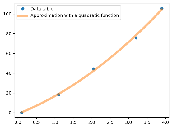

Let us also look at the approximation error:

e_i=y_i - f(x_i)

(27)

for $i=0,1,2,\dots,n-1$ .

With a correctly performed approximation, some $e_i$ are positive and some negative. Let us check whether this is true in our case:

e = y - apr_polynomial(x, a)
e

array([-0.06824269, -0.62517387, 2.1057209 , -2.69396374, 1.28165939])

Note: the higher the degree of the polynomial we use, the greater the probability of poor conditioning. For this reason we do not overdo the polynomial degree (in practice we mainly use low degrees)!

Using `numpy` for polynomial approximation¶

Let us look at how to use the numpy library for polynomial approximation.

First we use the function numpy.polyfit (documentation):

polyfit(x, y, deg, rcond=None, full=False, w=None, cov=False)

which requires three parameters: x and y represent the data table (also possible as lists of vectors), and deg is the polynomial degree. The remaining parameters are optional (e.g., w to use weights in the approximation).

The polyfit function returns a list of polynomial coefficients (highest order first); the result can also be a list of lists (if the input data is a list of vectors).

Note: numpy.polyfit and numpy.poly1d belong to the older interface for polynomials; for new programs numpy recommends the class numpy.polynomial.Polynomial (documentation): p = Polynomial.fit(x, y, deg=2) returns an object that we call as a function (p(x)), and p.convert().coef gives the coefficients in increasing order of powers (exactly the opposite of polyfit).

Let us look at its use for the example treated previously:

coef = np.polyfit(x, y, deg=2)
coef

array([ 3.17760897, 14.67380042, -1.21091344])

a # result of our own implementation

array([ 3.17760897, 14.67380042, -1.21091344])

Once we have the coefficients, we can create a polynomial object by calling numpy.poly1d (documentation):

poly1d(c_or_r, r=False, variable=None)

where c_or_r represents the list of polynomial coefficients, or the roots of the polynomial if r=True. The function returns an instance of the object, by calling which we can compute the values of the approximating polynomial at x, but we can also compute other things, such as the roots of the polynomial.

Let us look at an example:

p = np.poly1d(coef) # p is an instance of the poly1d object. We now obtain the approximation with y = p(x).

Let us plot the values:

plt.plot(x, y, 'o', label='Data table')
plt.plot(x_g, p(x_g), lw=5, alpha=0.5, label='Approximation with a quadratic function')
plt.legend();

Let us compute the roots of the polynomial:

p.roots

array([-4.69897273, 0.08109792])

Approximation with an arbitrary function¶

In approximation we are not limited to polynomials only. We can approximate data tables:

with a linear combination of linearly independent basis functions, or
with a function in which the parameters appear in a nonlinear relationship (e.g., $a_0\,\sin(a_1\,x+a_2)$ ).

For details, see the reference J. Petrišič: Uvod v Matlab za inženirje, Fakulteta za strojništvo 2013, p. 145.

We will focus on using the scipy package for approximation with a nonlinear function, which is based on the least-squares method.

Approximation with a harmonic function¶

The data table is defined as:

x = np.array([ 0.1, 0.8, 1.7, 2.5, 3.4, 4.2,  5.1])
y = np.array([ 0.01, -1.13, 0.02, 0.92, -0.01, -0.98, 0.1])

Let us plot the data table:

plt.plot(x, y, 'o', label='Data table')
plt.legend();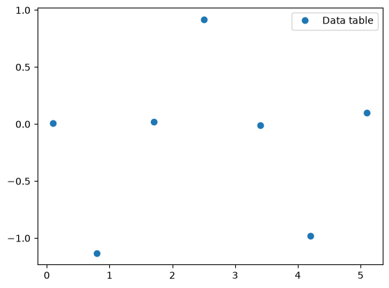

We will perform the approximation with a nonlinear function using scipy.optimize.curve_fit (documentation):

curve_fit(f, xdata, ydata, p0=None, sigma=None, absolute_sigma=False, check_finite=True, bounds=(-inf, inf), method=None, jac=None, **kwargs)

which requires three parameters: f represents the definition of the Python function with which we want to approximate, and whose parameters we vary using the least-squares method. xdata and ydata represent the data table. It is also recommended to define an estimate of the sought parameters p0. The remaining parameters are optional.

The function returns two arrays: popt, which represents the parameters found, and pcov, which represents the estimated covariance of popt.

First let us define a Python function whose first parameter is the independent variable x, followed by the parameters we want to determine:

def func(x, A, ω, ϕ):
    return A*np.sin(ω*x+ϕ)

where A is the amplitude, ω the angular frequency, and ϕ the phase of the harmonic function. With the help of the figure we can guess the initial estimates: A=1, ω=1, ϕ=0

Now we import curve_fit and run the optimization procedure:

from scipy.optimize import curve_fit

popt, pcov = curve_fit(func, x, y, p0=[1, 1, 0])
popt

array([ 1.01461945, 1.89652046, -3.27943097])

We have computed the expected values (see above).

func(x, *popt)

array([-0.0525477 , -0.99608783, -0.05612665,  1.00860622, -0.02753942,
       -1.01426499,  0.1110182 ])

x_g = np.linspace(np.min(x), np.max(x), 50)
y_g = func(x_g, *popt) # note how we passed the parameters to the function
plt.plot(x, y, 'o', label='Data table')
plt.plot(x_g, y_g, label='Approximation')
plt.legend();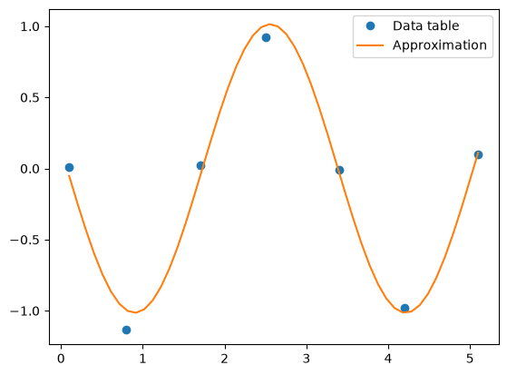

Additional¶

Make an .exe of your program:

Take a look at the pandas package. Pandas

Approximation with splines using `SciPy`¶

Let the data table be:

x = np.linspace(-3, 3, 20)
x

array([-3.        , -2.68421053, -2.36842105, -2.05263158, -1.73684211,
       -1.42105263, -1.10526316, -0.78947368, -0.47368421, -0.15789474,
        0.15789474,  0.47368421,  0.78947368,  1.10526316,  1.42105263,
        1.73684211,  2.05263158,  2.36842105,  2.68421053,  3.        ])

np.random.seed(0) # seed of the random number generator
y = np.exp(-x**2) + 0.1 * np.random.normal(scale=.5, size=len(x))
y

array([ 0.08832603,  0.02075073,  0.0526001 ,  0.12684217,  0.14234432,
        0.08387244,  0.34226064,  0.52862107,  0.79385312,  0.99590738,
        0.98257964,  0.87172774,  0.57424082,  0.30083997,  0.15492949,
        0.06565014,  0.08950146, -0.00659471,  0.01639626, -0.04258138])

Let us look at the object scipy.interpolate.UnivariateSpline (documentation), which enables both interpolation and approximation with splines:

UnivariateSpline(x, y, w=None, bbox=[None, None], k=3, s=None, ext=0, check_finite=False)

The parameters x and y represent the data table.

Note: UnivariateSpline has been marked as legacy since SciPy 1.15; the more modern equivalent for approximation (smoothing) with splines is scipy.interpolate.make_smoothing_spline (documentation) or make_splrep. The object interface below still works and is clearer for learning.

The optional parameter s sets the value that the sum of squares of the differences between the approximating spline and the approximation points must not exceed:

sum((w[i] * (y[i]-spl(x[i])))**2, axis=0) <= s

w are the weights of the individual points.

If we set s=0, we require interpolation.

The parameter k defines the degree of the polynomial spline (the default is k=3).

We perform approximation with splines by defining, in addition to the data table x and y, the parameter s as well. Let us perform interpolation:

from scipy.interpolate import UnivariateSpline
spl = UnivariateSpline(x, y, s=0.)

x_g = np.linspace(-3, 3, 100)
plt.plot(x, y, 'o', ms=5, label='Approximation points')
plt.plot(x_g, spl(x_g), lw=3, label='Spline', alpha=0.6)
plt.legend();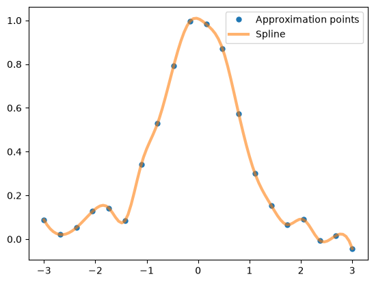

Let us also perform the approximation:

spl_a = UnivariateSpline(x, y, s=.1)

plt.plot(x, y, 'o', ms=5, label='Approximation points')
plt.plot(x_g, spl(x_g), lw=3, label='Interpolation (s=0)');
plt.plot(x_g, spl_a(x_g), lw=3, label='Approximation (s=0.1)');
plt.plot(spl_a.get_knots(), spl_a(spl_a.get_knots()), 'o', label='Knots in the approximation');
plt.legend();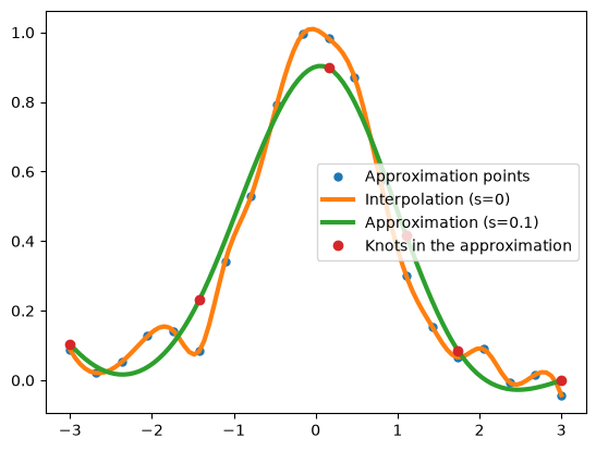

The actual residual:

spl_a.get_residual()

0.10002662427563205

Introduction¶

Least-squares method for a linear function¶

Using the pseudo-inverse matrix¶

Least-squares method for an arbitrary polynomial¶

Numerical example¶

Using numpy for polynomial approximation¶

Approximation with an arbitrary function¶

Approximation with a harmonic function¶

Additional¶

Approximation with splines using SciPy¶

Using `numpy` for polynomial approximation¶

Approximation with splines using `SciPy`¶