Introduction to Python#
What is the Python ecosystem?#
Many readers find the word ecosystem confusing. The Dictionary of the Slovenian Literary Language today recognizes only the usage related to ecology. In computer science, however, over the past few decades the word ecosystem has also been used in the context of the so-called digital ecosystem; in the case of Python this means the entire collection of different packages (pypi.org alone currently hosts more than 685 thousand different packages) that are built on the Python programming language and are interconnected.
The Python ecosystem is much more than just the Python programming language! In the first four lectures, this book focuses on the part of this ecosystem that is interesting and useful primarily for engineering professions.
Python is a high-level programming language, with a high level of abstraction. Low-level programming languages, in contrast, have a low level of abstraction (e.g., machine code).
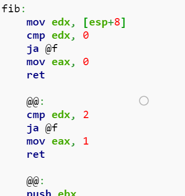
Let us look at the computation of a Fibonacci number, which follows the definition:
Computation of \(F_n\) in machine code:
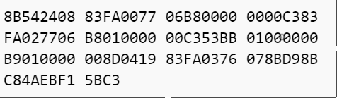
MASM code
C
int Fibonacci(int n)
{
   if ( n == 0 )
      return 0;
   else if ( n == 1 )
      return 1;
   else
      return ( Fibonacci(n-1) + Fibonacci(n-2) );
}
Python
def fib(n):
    if n == 0:
        return 0
    elif n == 1:
        return 1
    else:
        return fib(n-1) + fib(n-2)
numbers = [1., 2, 3, 4, 5] # list of numbers
[number**2 for number in numbers if number>3]
[16, 25]
Python enables a high level of abstraction and therefore abstract code. Now we will look at an example of Python code:
numbers = [1, 2, 3, 4, 5] # list of numbers
[number for number in numbers if number%2]
Even though at this point we do not yet have enough knowledge, let us try to understand/read it:
the first line defines a list of numbers; everything that follows the # character is a comment
the result of the second line is a list, which is defined by the square brackets; inside the brackets we read:
return
numberfor each (for)numberin (in) the listnumbers, if (if) dividingnumberby 2 leaves a remainder of 1.
We can see that the level of abstraction really is high, since we needed a lot of words to explain the content!
Let us look at the result:
numbers = [1, 2, 3, 4, 5] # list of numbers
[number for number in numbers if number%2]
[1, 3, 5]
A brief overview of the beginnings of some programming languages:
1957 Fortran, * 1970 Pascal, * 1972 C
1980 C++, * 1984 Matlab, * 1986 Objective-C
1991 Python, * 1995 Java, * 1995 Delphi
2006 Rust, 2009 Go, 2012 Julia
Who learns Python, and why use it?#
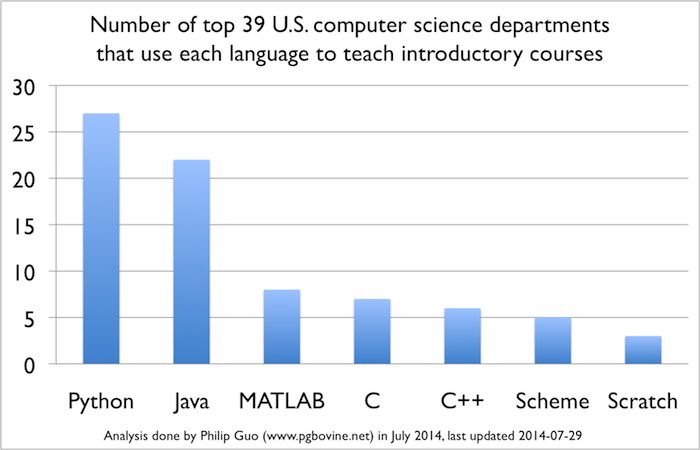
USA
Python is the language most often taught at the best American universities.
At the University of Berkeley at the start of the 2017/18 academic year (more than 1200 students in the Data science course, which is based on the Jupyter notebook technology).
%%html
<blockquote class="twitter-tweet" data-lang="en"><p lang="en" dir="ltr">First day of class in Foundations of <a href="https://twitter.com/hashtag/Datascience?src=hash">#Datascience</a> for <a href="https://twitter.com/BerkeleyDataSci">@BerkeleyDataSci</a> - all materials at <a href="https://t.co/yyoJbaKlnL">https://t.co/yyoJbaKlnL</a> <a href="https://t.co/J6DLd0VQTl">pic.twitter.com/J6DLd0VQTl</a></p>— Cathryn Carson (@CathrynCarson) <a href="https://twitter.com/CathrynCarson/status/900408152348270592">August 23, 2017</a></blockquote>
<script async src="//platform.twitter.com/widgets.js" charset="utf-8"></script>
First day of class in Foundations of #Datascience for @BerkeleyDataSci - all materials at https://t.co/yyoJbaKlnL pic.twitter.com/J6DLd0VQTl
— Cathryn Carson (@CathrynCarson) August 23, 2017
Over the past 10 years Python has been rapidly gaining popularity and is today one of the best (IEEE Spectrum.) and also one of the most popular programming languages (Why is Python Growing so Quickly? and Python’s explosive growth).
Uses of Python?#
Some international companies: Nasa, Google, Cern.
Some companies in Slovenia: Gorenje, Kolektor, Iskra Mehanizmi, Hidria, Mahle, Domel, ebm-papst Slovenia, Efaflex…
More and more programs have built-in scripting support for Python: Abaqus, Ansys Workbench, MSC (Adams, SimXpert), MS Excel, ParaView, LMS Siemens, AVL.
Some commercial programs written in Python: BitTorrent, Dropbox.
An extensive list is available here.
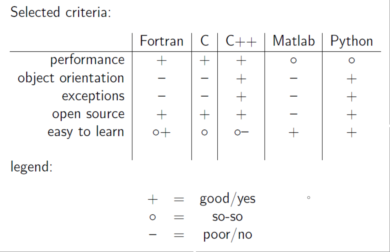
Python vs Matlab#
In the past, Matlab was often taught at universities and also had many users in industry. For years now, the Python ecosystem has been a substantially more powerful tool for most tasks. You will find a huge number of comparisons online, e.g.: Python vs Matlab.
A short comparison based on this source:
The syntax is generally very similar. An important difference is that in Matlab indices start at 1, while in Python they start at 0.
If you are younger than 25-30 years, you can probably skip the rest of this cell.
If you are not, you probably learned Matlab and are wondering why your club has fewer and fewer members. It is probably time to switch to Python; here is an article that can help you: MATLAB vs Python: Why and How to Make the Switch.
Installing Python#
Go to www.python.org and install Python; make sure to choose version 3.10 or newer (64 bit). Follow the prepared video instructions.
Using the GitHub repository and updates#
This book is continuously being updated; the latest version is available at:
in source form at github.com/jankoslavic/pynm,
in web form at https://jankoslavic.github.io/pynm.
To synchronize with the online repository, it is best to use one of the Git clients, e.g., GitHub Desktop or the one within Visual Studio Code (presented later). Git is, in fact, a very powerful tool and allows a group of developers to work relatively easily on the same code and to keep control over different versions of the files.
Visual Studio Code#
In this course we will mostly program in Jupyter Lab/Notebook within Visual Studio Code - VSC, which enables very efficient programming using fully formatted text and interactive displays. To install VSC, follow the prepared video instructions.
When we want to program more extensive and more generally useful packages and dedicated programs, we usually also make use of other features that the VSC integrated development environment (IDE) offers. In recent times VSC has been gaining popularity because of its speed, ease of use, and extensibility. How VSC can help us with programming is shown excellently in a video on the topic of productivity with VSC.
Installing add-ons and updates#
pypi.org hosts many different packages! We install them from the command prompt* using the pip command.
* You can open the command prompt in the Windows operating system by clicking "Start" and typing "command prompt" and pressing "enter", or by opening a terminal within VSC (video).
We will look at the details of installing add-ons next time. To make sure you have the latest version of the packages, do the following:
Open the command prompt,
run the command to update the packages we will need throughout the course:
pip install numpy scipy matplotlib sympy requests jupyter --upgrade
Jupyter notebook (Jupyter lab)#
Jupyter notebook is an interactive environment that works as a web application and can be used with various programming languages (e.g., Python, Julia, R, C, Fortran … the name JuPyt[e]R was also formed from the first three).
The easiest way to try out Jupyter notebook is here: try.jupyter.org or colab.research.google.com.
We start Jupyter notebook (in any folder) from the command prompt or from the File Explorer with the command:
jupyter notebook,
or within VSC as presented in the video.
Notes:
by running
jupyter labwe get an upgrade of thejupyter notebookenvironment (a slightly more demanding environment, but a substantially more advanced one),here we assume that the path to the jupyter[.exe] file is added to the environment variables (and that you can run it from the command prompt in any folder),
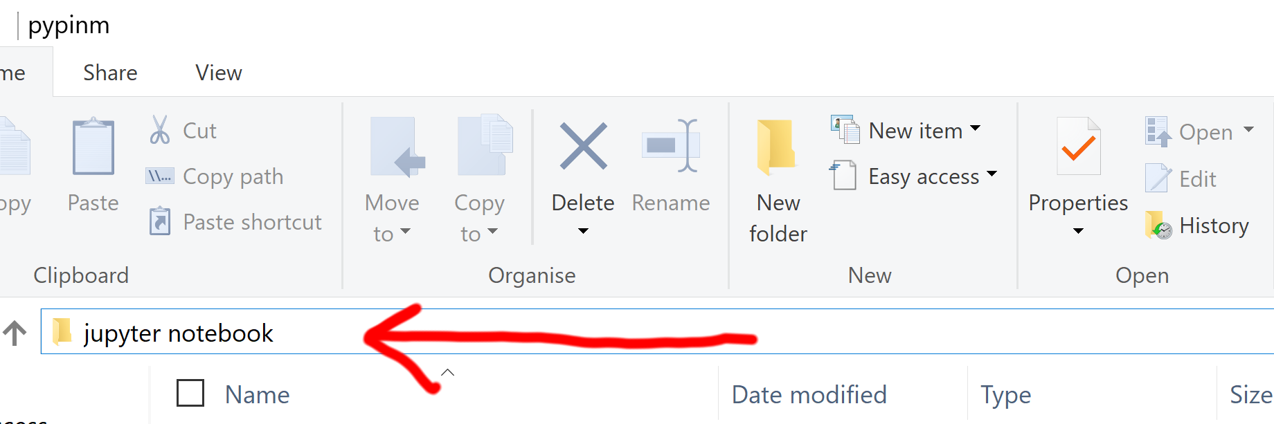
if you want to open the command prompt in any folder, then in the File Explorer hold
shiftand right-click the folder; then choose Open command window here.
We access the Jupyter server through a web browser. First you are shown a list of folders and files you can access within the folder in which you ran the command jupyter notebook. Then look for the new icon in the upper-right corner and click Python 3. This will start your first Jupyter notebook (with a Python kernel). Find the menu bar and on the right side click Help and then User interface tour. Also take a look at Help/Keyboard shortcuts.
A Jupyter notebook is composed of so-called cells.
A cell has two states:
Command mode: this state is entered by pressing [escape],
Edit mode: this state is entered by pressing [enter].
In both cases a cell is executed by pressing [shift + enter].
Cells can be of different types; here we will use two types:
Code: in this case the cell contains program code (the shortcut in command mode is the [y] key),
Markdown: in this case the cell contains text formatted according to the Markdown standard (the shortcut in command mode is the [m] key).
Markdown#
Jupyter notebook allows writing in markdown mode, which was introduced in 2003-2004 by John Gruber. The purpose of markdown is for the writer to focus on the content, while using a few simple rules for formatting. Later, markdown can be converted into web form, into pdf (e.g., via LaTeX), etc. The essential rules (related mainly to use on GitHub) are given here; below we will briefly review them.
We define headings with the # character:
# means a first-level heading,
## means a second-level heading, etc*.
* If you look at the code, you notice that the \ character appears before the # character so that the # character itself is displayed and its function for a first-level heading is not used. The same applies to other special characters.
Text formatting is defined by special characters; if we want a word (or several words) in italic form, we have to place such text between two * characters: the text in edit mode in the form *example* would be displayed as example.
Overview of the symbols that define the format:
italic:*
bold: **
~~strikethrough~~: ~~
symbol: `functions: ``code block: ```.
Note: for an example of a Python code block, see the introductory section, the Fibonacci example.
Within markdown we can also use LaTeX syntax. LaTeX is a very powerful system for text editing; at the Faculty of Mechanical Engineering, University of Ljubljana, the templates for diploma theses are prepared in LaTeX and in Word. Here we will use LaTeX only for writing mathematical expressions.
There are two modes:
inline mode: starts and ends with the \\( character, example: \)a^3=\sqrt{365}$,
block mode: starts and ends with the two characters \\(\\\), example: $\(\sum F=m\,\ddot{x}\)$
Above we have already used lists, which we begin with the * character on a new line:
we can write lists
with several levels
3rd\(.\) level
2nd\(.\) level
we can write italic
we can write bold.
If we want numbered lists, we start with “1.” and then continue with “1.”:
first element
second
next …
We can also include html (Hypertext Markup Language) syntax in the document. The simplest thing to include as html are images.
We use:

For display:

We can also include external resources (e.g., a video from YouTube). Since this is a potential security risk, we do not do it in a markdown cell as above, but in a code cell, using the so-called magic command %%html, which defines that the entire block will be in html syntax (by default, code cells contain Python code):
%%html
<iframe width="560" height="315" src="https://www.youtube.com/embed/VLcPd07-gnk" frameborder="0" allowfullscreen></iframe>
There are many more magic commands in the notebook (see the documentation), and we will learn some of them later, when we need them!
So far we have already several times used references to external resources; we do it like this:
[Link name](address of the resource)
Example: [Website of the Ladisk laboratory](www.ladisk.si) is formatted as: Website of the Ladisk laboratory.
Within markdown we can prepare simple tables. Preparation is relatively easy: we simply insert vertical bars | between the words where the vertical line should be. The header row is followed by a row that defines the alignment in the table.
Example:
| Name   | Mass [kg]  | Height [cm]  |
|:-|-:|:-:|
| Lakotnik  | 180  | 140  |
| Trdonja | 30  | 70  |
| Zvitorepec  | 40  | 100  |
Results in:
Name |
Mass [kg] |
Height [cm] |
|---|---|---|
Lakotnik |
180 |
140 |
Trdonja |
30 |
70 |
Zvitorepec |
40 |
100 |
We notice that the colon defines the alignment of the text in the column (left :-, right -:, or centered :-:).
First program and PEP#
Now we are ready for the first program written in Python:
a = 5.0
print(a)
We can write the program in any text editor (e.g., Notepad) and save it in a file name.py.
Example code in the Visual Studio Code environment:
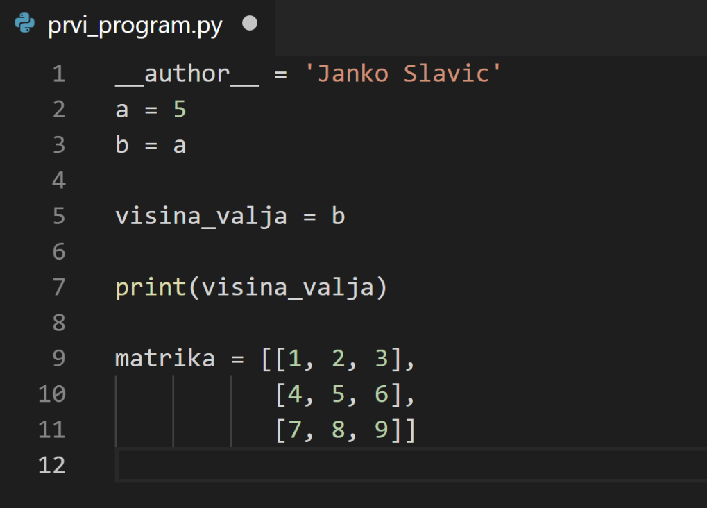
We then run this file in the command prompt (we assume that the path to the python.exe file is added to the environment variables; otherwise see this source):
python name.py
>>> 5.0
With the characters >>> we denote the result that we get in the command prompt.
The above example of executing a Python program represents the so-called classic way of running programs from beginning to end. Here we will more often use the so-called interactive way, where we execute code within an individual code cell:
a = 5.0  # this is a comment
print(a) # prints the value of a
5.0
PEP - Python Enhancements Proposal#
Python has high standards regarding quality and aesthetics. Early in the development of the language, the principle of proposing improvements through the so-called Python Enhancements Proposal (PEP for short) became established.
PEP8#
One of the more important ones is PEP8, which defines style:
indentation: 4 spaces,
one space around the operator
=, that is:a = 5and nota=5,variable and function names should be descriptive, written with underscores:
cylinder_width = 5,for classes we use the so-called CamelCase format.
for arithmetic operators we place spaces by feel:
x = 3*a + 4*borx = 3 * a + 4 * b,there is no space after an opening parenthesis or before a closing parenthesis, and likewise no space before a parenthesis when calling a function:
x = sin(x), but notx = sin( x )orx = sin (x),a space after a comma:
range(5, 10)and notrange(5,10),no spaces at the end of a line or in an empty line,
within a function we can occasionally add a single empty line,
between functions we place two empty lines,
we import (
import) each module on a separate line,first we import the standard Python libraries, then other libraries (e.g., numpy), and finally our own.
Note: modern development tools help us format code that conforms to PEP8 (in VSC press ctrl+shift+P, type “Format document”, and press enter)!
PEP20#
PEP20 is the next important PEP, also called The zen of Python; these are guidelines that we try to follow when programming. Here we list only a few of the guidelines:
Beautiful is better than ugly.
Simple is better than complicated.
Flat is better than nested.
Readability counts.
Special cases aren’t special enough to break the rules.
If the implementation is hard to explain, it’s probably a bad idea; if it’s easy to explain, it may be a good one.
Python basics#
Basic data types and operators#
Dynamic typing#
Python is a dynamically typed language. Variable types are not checked. As a consequence, some operations are not possible on certain types, or are adapted to the data type (later, for example, we will look at multiplying a string of characters). The type is determined upon assignment of a value; let us look at an example:
a = 1 # this is a comment: a is an integer
a
1
We display the type with the command type:
type(a)
int
We can overwrite the value of a with a new value:
a = 1.0  # this is now a floating-point number (float)
a        # if we write `a` like this on the last line, the value will be printed
1.0
type(a)
float
To print a value we can also use the function print(), which we will get to know in more detail later:
print(a)
1.0
We can call the documentation of a function by pressing [shift + tab]. E.g.: we write pri and press [shift + tab], and the help will appear in a pop-up window; if we hold [shift], an additional press of [tab] shows extended help, and a further double press of [tab] (so four times in total) shows the help in a new window.
We can also access help by placing ? before the function (for help) or ?? (which also shows the source code, if available).
Example:
?print
??print
Logical operators#
The logical operators are (source):
or, example:a or b; note: the second element is checked only if the first is not true,and, example:a and b; note: the second element is checked only if the first is true,not, example:not a; note: the non-logical operators have precedence:not a == bis interpreted asnot (a == b).
Comparison operators#
The comparison operators (source):
<less than,<=less than or equal,>greater than,>=greater than or equal,==equal,!=not equal,isidentity of the object of the compared operands,is notwhether the operands are not the same object.
Example:
5 < 6
True
We can make a chain of logical operators:
1 < 3 < 6 < 7
True
let us check identity (whether it is the same object):
a = 1
a == 1
True
Let us also use a logical operator:
1 < 3 and 6 < 7
True
1 < 3 and not 6 < 7
False
Here it is worth pointing out that in logical expressions, in addition to False, the value 0, None, an empty list (or string, tuple, …) are also falsy; everything else is True.
Let us look at a few examples:
1 and True
True
0 and True
0
(1,) and True
True
Data types for numeric values#
We will look at the most common data types that we will use later (source):
intfor representing an arbitrarily large integer,floatfor representing floating-point numbers,complexfor representing numbers in complex form.
We will get to know the data types in more detail (representation accuracy and the like) in the introduction to numerical methods.
Examples:
whole_number = -2**3000         # `**` represents the power operator
rational_number = 3.141592
complex_number = 1 + 3j     # `3j` represents the imaginary part
Operators on numeric values#
Data types sorted by increasing priority (source):
x + ysum,x - ydifference,x * yproduct,x / ydivision,x // yinteger division (the result is an integer rounded down),x % yremainder of integer division,-xnegation,+xunchanged,abs(x)absolute value,int(x)integer of typeint,float(x)rational number of typefloat,complex(re, im)complex number of typecomplex,c.conjugate()complex conjugate number,divmod(x, y)returns the pair(x // y, x % y),pow(x, y)returnsxto the powery,x ** yreturnsxto the powery.
For arithmetic operators it is worth pointing out the variant in which the result is assigned to the operand (source). This is called augmented assignment.
Let us look at an example. Instead of:
a = 1
a = a + 1 # we add the value 1
a
2
we can write:
a = 1
a += 1
a
2
Bit-level operators#
We will rarely use bit-level operators in engineering practice; nevertheless, let us list them by increasing priority (source):
x | ybitwise or ofxandy,x ^ yexclusive or (only one, not both) at the bit level ofxandy,x & ybitwise and ofxandy,x << nshift the bits ofxbynbits to the left,x >> nshift the bits ofxbynbits to the right,~xnegate the bits ofx.
Let us look at an example (source):
a = 21  # 21 in bit form: 0001 0101
b = 9   # 9 in bit form:  0000 1001

c = a & b; # 0000 0001 in bit form represents the number 1 in decimal
c
1
Let us display the number in bit form:
bin(c)
'0b1'
Composite data structures#
String#
A string is composed of characters according to the Unicode standard. We will not go into the details; it is important to note that, starting from version 3, Python made great progress (source), and that we can use arbitrary characters from the Unicode standard both in text and in program files .py.
A string starts and ends with a double “ or single ‘ quotation mark.
b = 'text' # b is a string
b
'text'
Here there are no problems with names that we are more used to:
π = 3.14
The character \(\pi\) is written in the notebook by typing \pi (the names are usually the same as those used in LaTeX) and then pressing [tab].
Some operations on strings:
print('short ' + b) # addition
print(3 * 'This is string multiplication. ')      # string multiplication
print('Integer:', int('5') + int('5'))      # conversion of the string '5' to an integer
print('Floating-point number:', float('5') + float('5'))  # conversion of the string '5' to a floating-point number
short text
This is string multiplication. This is string multiplication. This is string multiplication.
Integer: 10
Floating-point number: 10.0
Tuple#
Tuples (source) are lists of arbitrary objects that we separate with a comma and write inside round parentheses:
tuple_1 = (1, 'programming', 5.0)
tuple_1
(1, 'programming', 5.0)
We have already used the word object several times. What is an object? We will look at objects and classes in more detail later; for now we are satisfied with the fact that an object is more than just a name for a certain value; an object also has methods.
E.g., the second element is of type str, which also has the method replace for replacing characters:
tuple_1[1].replace('r', '8')
'p8og8amming'
If a tuple has only one object, then we have to end it with a comma (otherwise it is not distinguished from the object in parentheses):
tuple_2 = (1,)
type(tuple_2)
tuple
Tuples can also be written without round parentheses:
tuple_3 = 1, 'without parentheses', 5.
tuple_3
(1, 'without parentheses', 5.0)
We access objects in a tuple via the index (they start at 0):
tuple_1[0]
1
A tuple cannot be changed (it is immutable); we cannot remove or add elements. Calling the expression below would lead to an error:
tuple_1[0] = 3
>>> TypeError: 'tuple' object does not support item assignment
List#
Lists (source) are written similarly to tuples, but square brackets are used:
my_list = [1., 2, 'd']
my_list
[1.0, 2, 'd']
Unlike tuples, lists can be changed:
my_list[0] = 10
my_list
[10, 2, 'd']
Lists are mutable, and one has to be aware that the name in fact points to a location in the computer’s memory:
b = my_list
b
[10, 2, 'd']
Now b also points to the same location in memory.
Let us see what happens to my_list if we change an element of the list b:
b[0] = 9
b
[9, 2, 'd']
my_list
[9, 2, 'd']
If we want to make a copy of the data, then we have to do it like this:
b = my_list.copy()
b[0] = 99
b
[99, 2, 'd']
my_list
[9, 2, 'd']
Example of a list of lists:
matrix = [[1, 2, 3],
          [4, 5, 6],
          [7, 8, 9]]
matrix
[[1, 2, 3], [4, 5, 6], [7, 8, 9]]
We will learn more about matrices later.
Selected operations on lists#
Here we will look at some of the most common operations; for more, see the documentation.
First let us look at adding an element:
my_list = [0, 1, 'test']
my_list.append('adding an element')
my_list
[0, 1, 'test', 'adding an element']
Then inserting at a specific position (at index 1; the other elements are shifted):
my_list.insert(1,'to the second position')
my_list
[0, 'to the second position', 1, 'test', 'adding an element']
Then we can remove a specific element. We do this with my_list.pop(i) or del my_list[2]. The first way returns the removed element, the second only removes the element:
removed_element = my_list.pop(2) # remove the element with index 2 and return it
## the command: del my_list[2] would have a similar effect
print('list:', my_list)
print('removed element:', removed_element)
list: [0, 'to the second position', 'test', 'adding an element']
removed element: 1
With the method .index(v) we find the first element with value v:
my_list
[0, 'to the second position', 'test', 'adding an element']
my_list.index('test')
2
Why use a tuple and not a list?#
Tuples cannot be changed, so their numerical implementation is substantially lighter (in the numerical sense) and memory can be used better. Consequently, tuples are faster than lists; in addition, we cannot change them by accident. For a broader answer, see this source.
Sets#
Sets are in principle similar to the sets we know from mathematics. Sets in Python (documentation), unlike the other composite structures:
do not allow duplicate elements and
do not have an ordered sequence (important, e.g., for correct use in loops).
It is worth emphasizing that adding an element and determining membership of an element in a set are very fast operations.
We create them with curly braces {} or with the command set():
A = {'a', 4, 'a', 2, 'z', 3, 3}
A
{2, 3, 4, 'a', 'z'}
If we want to get rid of duplicate elements in a list, a very simple way is to create a set from the list:
B = set([6, 4, 6, 6])
B
{4, 6}
We can use the typical mathematical operations on sets:
B - A # elements in B without elements that are also in A
{6}
A | B # elements in A or B
{2, 3, 4, 6, 'a', 'z'}
A & B # elements in A and B
{4}
A ^ B # elements in A or B, but not in both
{2, 3, 6, 'a', 'z'}
Dictionary#
A dictionary (documentation) can be defined explicitly with key : value pairs, separated by commas inside curly braces:
parameters = {'height': 5.2, 'width': 43, 'g': 9.81}
parameters
{'height': 5.2, 'width': 43, 'g': 9.81}
We access the value of an element by using the key:
parameters['height']
5.2
More often we use the methods:
values(), which returns the values of the dictionary,keys(), which returns the keys of the dictionary,items(), which returns a list of tuples (key, value); we will often need this in loops.
Example:
parameters.items()
dict_items([('height', 5.2), ('width', 43), ('g', 9.81)])
Dictionaries can be changed; e.g., we add an element:
parameters['centroid_position'] = 99999
parameters
{'height': 5.2, 'width': 43, 'g': 9.81, 'centroid_position': 99999}
We remove elements (similar to above, pop removes and returns the value, del only removes):
parameters.pop('centroid_position')
99999
parameters
{'height': 5.2, 'width': 43, 'g': 9.81}
Operations on composite data structures#
Most composite data structures allow the following operations (documentation):
x in sreturnsTrueif any element ofsis equal tox, otherwise returnsFalse,x not in sreturnsFalseif any element ofsis equal tox, otherwise returnsTrue,s + tconcatenatessandt,s * norn * sresults insrepeatedntimes,s[i]returns thei-th element ofs,s[i:j]returnssfrom elementi(inclusive) toj(not included),s[i:j:k]slicingsfrom elementitojwith stepk,len(s)returns the length ofs,min(s)returns the smallest element ofs,max(s)returns the largest element ofs,s.index(x[, i[, j]])returns the index of the first occurrence ofxins(from indexitoj),s.count(x)returns the number of elements.
Some examples:
'a' in 'abc' # in compares whether an object is in a string, list, ...
True
Above we had the dictionary parameters:
{'g': 9.81, 'height': 5.2, 'width': 43}
Let us check whether it contains an element with the key width:
'width' in parameters
True
Counting and slicing composite data structures#
Assume the string below:
alphabet = 'abcdefghijklmnoprstuvz'
In Python we start counting indices at 0! Online you can find discussions about whether it is correct for indices to start at 0 or 1. Why start at 0 is explained very nicely by Prof. Dr. Janez Demšar in the book Python za programerje (source, page 28), or also by Prof. Dr. Edsger W. Dijkstra in a note on the web.
We call slicing the operation in which we cut certain members out of a list.
The general rule is:
s[i:j:k]
which means that the list s is sliced from element i to j with step k. If we do not provide one of the elements, then the (default) value is used:
idefaults to 0, which means the first element,jdefaults tolen(s)(the sequence length), which means the last element is also included,kdefaults to 1.
The first character is therefore:
alphabet[0]
'a'
The first three characters are:
alphabet[:3]
'abc'
Of the first 15 characters, every third one is:
alphabet[:15:3]
'adgjm'
The last fifteen characters, every third one:
alphabet[-15::3]
'hknru'
When we want to reverse the order, we can do it like this (we read from the beginning to the end with step -1, which means from the end toward the beginning with step 1:)):
alphabet[::-1]
'zvutsrponmlkjihgfedcba'
Program flow control#
We will look at some basic tools for controlling the flow of program execution (documentation).
The if statement#
A typical form of the if statement (documentation):
if condition0:
    print('condition0 was satisfied')
elif condition1:
    print('condition1 was satisfied')
elif condition2:
    print('condition2 was satisfied')
else:
    print('No condition was satisfied')
Example:
a = 6
if a > 5:
    print('a is more than 5') # executes if the condition is true.
    print(13*'-')
a is more than 5
-------------
Above we indented the function print, since it belongs to the block of code that executes in the case a > 0. Some programming languages put the code inside a block in curly or other brackets and additionally indent it. In Python it is only indented. The indentation is typically 4 spaces. It can also be a tab (less common), but within a single .py file we may use only one indentation method.
We can also write statements on a single line, but such use is discouraged, since it reduces the readability of the code:
if a > 5: print('this form is discouraged'); print(40*'-'); print('using a semicolon instead of a new line')
this form is discouraged
----------------------------------------
using a semicolon instead of a new line
The if expression#
In addition to the if statement, Python also has an if expression (the ternary operator, see the documentation).
The syntax is:
[execute if True] if condition else [execute if False]
A simple example:
'It is true' if 5==3 else 'It is not true'
'It is not true'
If expressions are very useful, and we will often use them in list comprehensions!
The while loop#
The syntax of the while loop (documentation) is:
while condition:
    [code to execute]
else:
    [code to execute]
Here it should be emphasized that the else part is optional and executes upon exiting the while loop. The break command interrupts the loop and does not execute the else part. The continue command interrupts the execution of the current code and goes immediately to testing the condition.
A simple example:
a = 0
while a < 3:
    print(a)
    a += 1
else:
    print('--')
0
1
2
--
The for loop#
In Python we will use the for loop very often (documentation). The syntax is:
for element in list_with_elements:
    [code to execute]
else:
    [code to execute]
Similar to while, here too the else part is optional.
Let us look at an example:
names = ['Jaka', 'Miki', 'Luka', 'Anja']
for name in names: # an assignment is hidden here; ``name`` gets a new value each time
    print(name)
Jaka
Miki
Luka
Anja
It is very useful to loop over dictionaries:
print('The dictionary is:', parameters)
for key, val in parameters.items():
    print(key, '=', val)
The dictionary is: {'height': 5.2, 'width': 43, 'g': 9.81}
height = 5.2
width = 43
g = 9.81
List comprehensions#
In programming we often encounter the need to perform operations on each individual element of a list. We have already learned the for loop, which we can use in such a case.
Let us look at an example where we compute the square of numbers:
my_list = [1, 2, 3] # source list
result = [] # prepare an empty list into which we will add the results
for element in my_list:
    result.append(element**2)
result
[1, 4, 9]
We can achieve the same result much more simply with so-called list comprehensions (see the documentation).
The above example would be:
my_list = [1, 2, 3] # source list
result = [element**2 for element in my_list] # <<< on the right-hand side of = is a list comprehension
result
[1, 4, 9]
A list comprehension is represented by the code [element**2 for element in my_list], which in fact says exactly what is written: compute the square for each element in the list. The square brackets indicate that the result is a list.
A list comprehension has the following syntax:
[code for element in list]
and it has primarily two advantages:
clarity / compactness of the code and
slightly faster execution.
We have already been able to judge the clarity/compactness. How do we check the speed? The easiest way to do this is with the so-called magic command %%timeit, that is, measure the time (see the documentation); below we will use the block magic command (denoted by %%):
%%timeit -n1000
where the parameter -n1000 limits the time measurement to 1000 repetitions.
First the longer way:
my_list = range(1000)
%%timeit -n1000
result = []
for element in my_list:
    result.append(element**2)
48.5 μs ± 305 ns per loop (mean ± std. dev. of 7 runs, 1,000 loops each)
Then the list comprehension (clearer and slightly faster):
%%timeit -n1000
result = [element**2 for element in my_list]
43.8 μs ± 1.4 μs per loop (mean ± std. dev. of 7 runs, 1,000 loops each)
Let us look at two more useful examples:
using the
ifexpression to compute a new value,using the
ifexpression to decide whether a new value is computed at all.
When computing a new value, we insert the if expression in the part before for:
my_list = [1, 2, 3]
[el+10 if el<2 else el**2 for el in my_list]
[11, 4, 9]
Often, however, we do not want to perform the computation at all for certain elements; in this case we insert the if expression after the list:
[el**2 for el in my_list if el >1]
[4, 9]
The zip function#
When we want to combine several lists in a loop, we use the zip function (documentation); example:
x = [1, 2, 3]
y = [10, 20, 30]

for xi, yi in zip(x, y):
    print('The pairs are: ', xi, 'and', yi)
The pairs are:  1 and 10
The pairs are:  2 and 20
The pairs are:  3 and 30
The range function#
We will often use the for loop together with the range function (documentation). The syntax is:
range(stop)
range(start, stop[, step])
So if we call the function with one parameter, it is stop: up to which number we count. In the case of a call with two parameters start, stop, we count from, to! The third parameter is optional and defines the step step.
Let us look at an example:
for i in range(3):
    print(i)
0
1
2
The enumerate function#
We also often use the for loop with the enumerate function, which numbers the elements (documentation).
Let us look at an example:
for i, name in enumerate(names):
    print(i, name)
0 Jaka
1 Miki
2 Luka
3 Anja
To conclude: a cheat sheet :)#
There are many of them; here is a link to one.
Some more reading: automatetheboringstuff.com.
And one tweet:
%%html
<blockquote class="twitter-tweet" data-lang="en"><p lang="en" dir="ltr">The most important slide from my <a href="https://twitter.com/PyData">@PyData</a> talk. <a href="https://t.co/Hc8j4ZpHV4">pic.twitter.com/Hc8j4ZpHV4</a></p>— Almar Klein (@almarklein) <a href="https://twitter.com/almarklein/status/708909917684568064">March 13, 2016</a></blockquote>
<script async src="//platform.twitter.com/widgets.js" charset="utf-8"></script>
The most important slide from my @PyData talk. pic.twitter.com/Hc8j4ZpHV4
— Almar Klein (@almarklein) March 13, 2016
Embedding a local video with transformations#
from IPython.core.display import HTML
HTML('<style>video{\
  -moz-transform:scale(0.75) rotate(-90deg);\
  -webkit-transform:scale(0.75) rotate(-90deg);\
  -o-transform:scale(0.75) rotate(-90deg);\
  -ms-transform:scale(0.75) rotate(-90deg);\
  transform:scale(0.75) rotate(-90deg);\
}</style>')
(The cell above does not display correctly on GitHub)
Exercise questions#
String#
Question 1: Write your first and last name as a string. Convert the string into a list and print it.
Question 2: Print the last character in the prepared list twenty times.
List, tuple#
Question 3: In Jupyter notebook, call up the help for the tuple function. Define a list with five different floating-point numbers and convert it into a tuple.
Question 4: Try to add a new element to the created tuple. Comment, convert the tuple into a list…
Question 5: Find the index of the largest element in the list and remove that element. If necessary, look up the help for the functions max, list.index.
Question 6: Prepare a new list by sorting the list from the previous problem by size and storing the first (smallest) three in a new list.
The zip function#
Question 7: Prepare a list of three strings: ['smallest', 'middle', 'largest'].
Using the zip and list functions, prepare a list of tuples from the list of strings and the list from the previous question.
Dictionaries#
Question 8: From the list of tuples in the previous problem, form a dictionary. Add a new key ‘negative’ to it and store an arbitrary negative number in it.
The if statement, for and while loops#
Question 9: Prepare a list of all odd divisors of an arbitrary natural number N greater than 100 that is not a prime number.
Question 10: For all natural numbers i less than or equal to 20 that are not in the list of divisors from the previous problem, write into a new list the remainder of integer division of N by i.
Question 11: Remove the duplicate elements from the above list of remainders.
Question 12: For all elements of the list from the previous problem, print the pair of the element and its index in the list, in the form index: element.
Question 13: Using a while loop, divide the number 1000 by 2 as many times as needed for the result to be less than \(10^{-3}\).
Print the number of division operations needed.